Pivots
Overview
You can use the pivot table in Analysis > Pivot. Most of the data collected by Logpresso Sonar consists of event information (logs) that occur in chronological order. By filtering only the necessary data from this time-ordered dataset and then swapping rows and columns into the desired format, you can identify relationships between items, perform aggregations, and gain meaningful insights through correlation analysis with other data. The pivot feature allows you to easily conduct advanced data analysis without having to write complex queries.
Screen Layout
Before Data Loading
When you navigate to Analysis > Pivot, you start with a blank screen as shown below. Items 1 to 3 are the work panel, and 4 is the workspace.
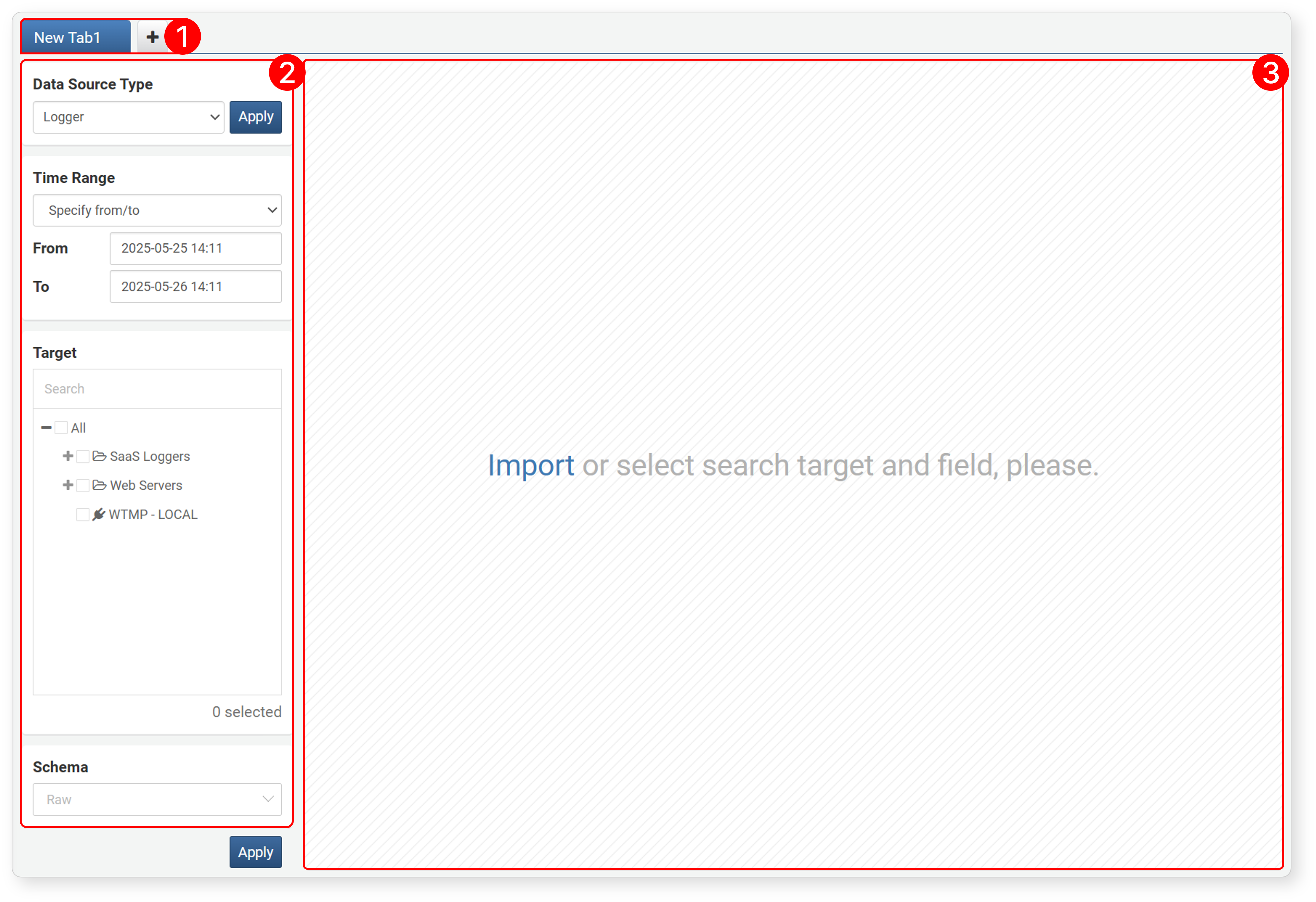
- 1. Tab
-
Pivot operations are performed in the tab screen. You can open new tabs to perform multiple pivot operations.
NoteIf you navigate away from the pivot screen, all tabs will be closed and not saved. If you want to keep your tabs, open the web console in a new window and use it there.
- 2. Data Loading Settings
-
Used to load data (loggers, tables, datasets, behavior profiles, events) for analysis.
-
When you select a Data Source Type, you can choose the analysis period, target/fields to query, and log schema according to the data type. Click Apply to display the data in the workspace.
- 3. Workspace
-
The area where data is displayed after executing data loading.
After Data Loading
After loading data, the screen layout changes as follows.
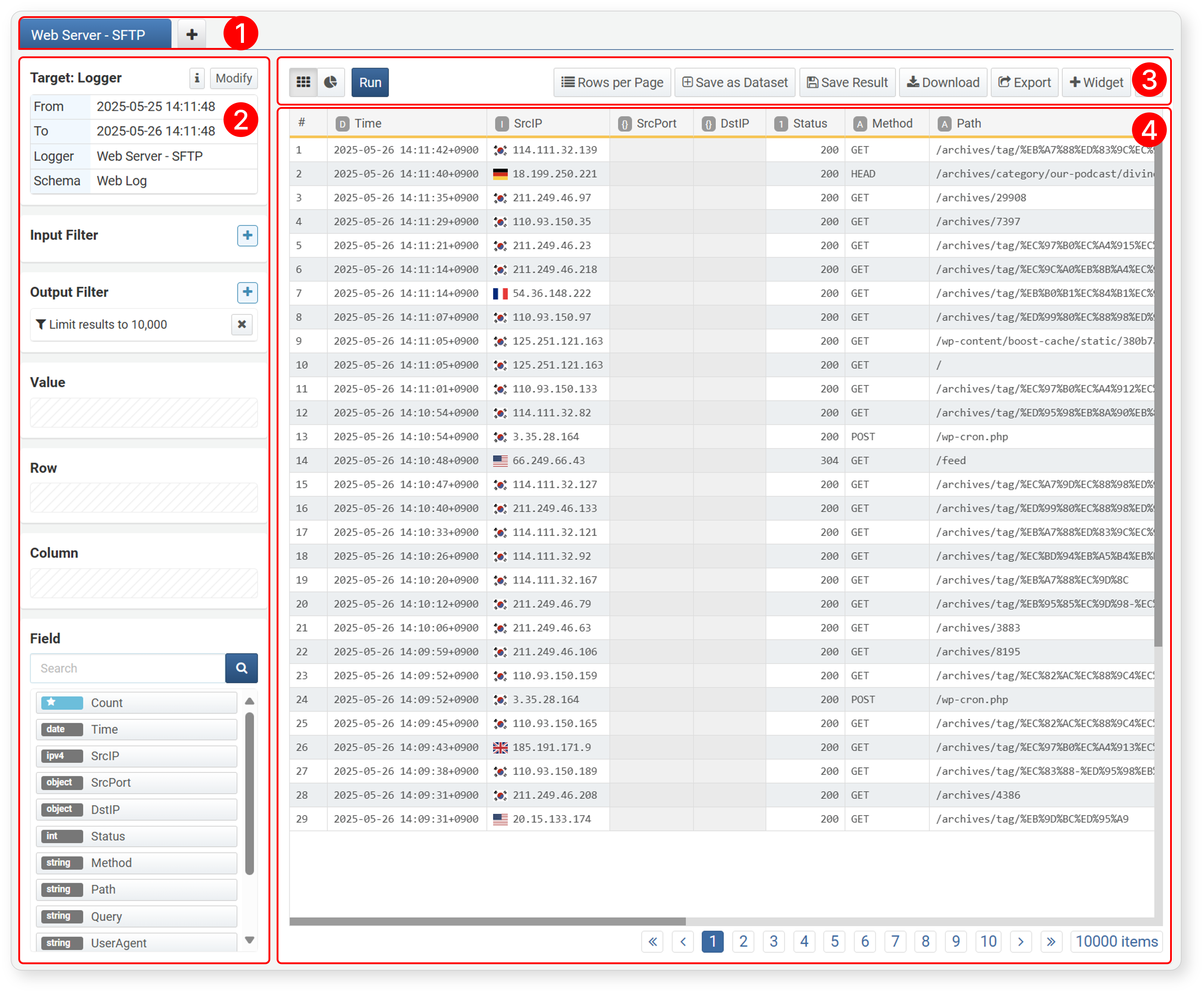
- 1. Tab
- After loading data, the tab shows the name of the target (except when data is loaded by directly entering a query).
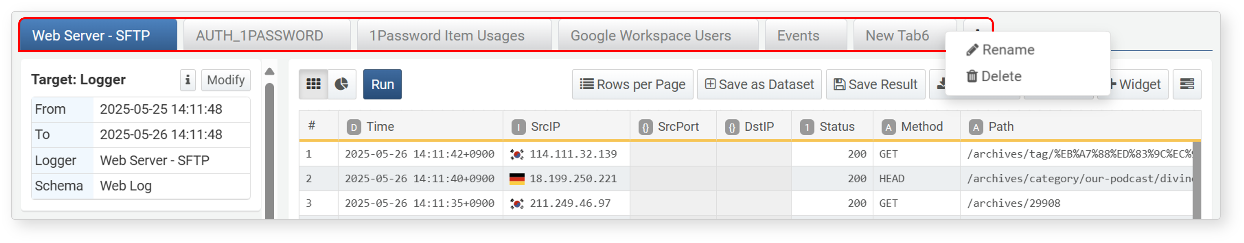
- When you move the cursor to the right of the tab name, a ∨ icon appears. Click it to open a popup menu where you can rename or close the tab.
- 2. Pivot Settings
- Displays input filters, result filters, values, rows, columns, and field tools for performing analysis tasks.
- 3. Toolbar
- Provides tools to view loaded data in a grid, convert queried data into dashboard widgets, and convert to datasets, query results, or pivot files.
- 4. Workspace
- The area where the data for analysis tasks is displayed.
Workflow
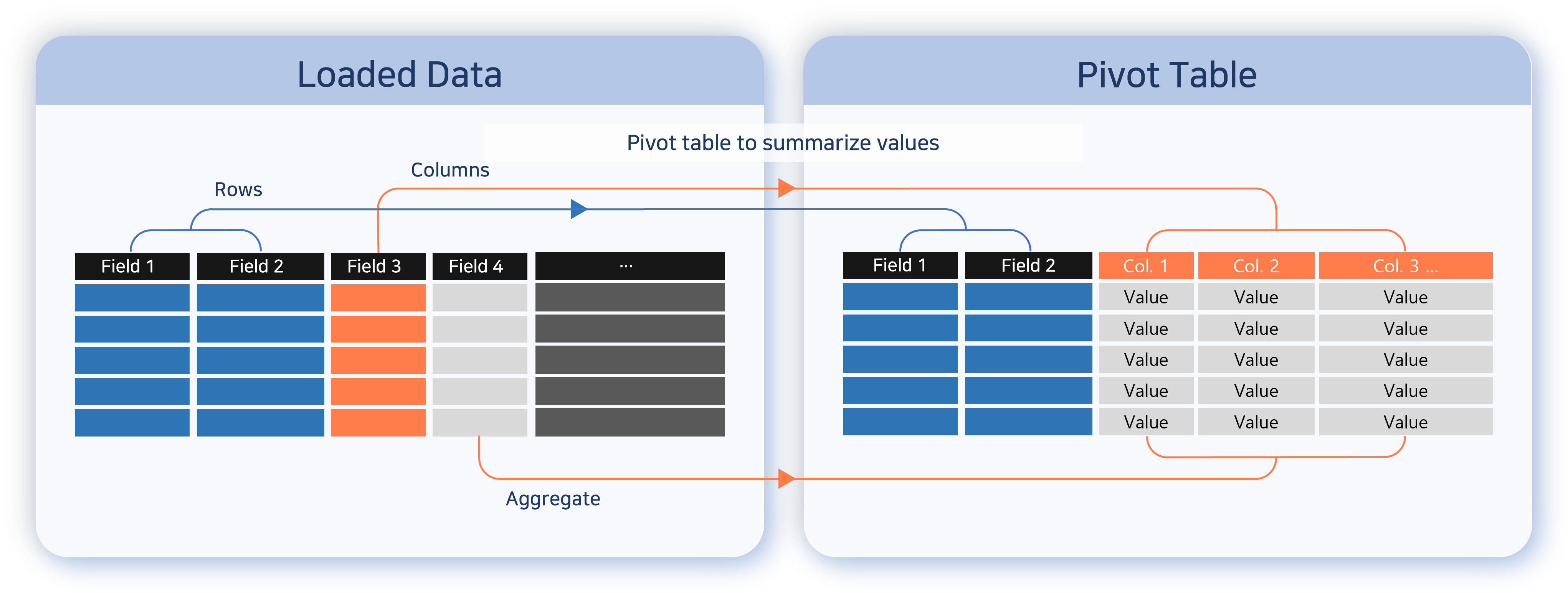
The following diagram illustrates the process of performing a pivot.
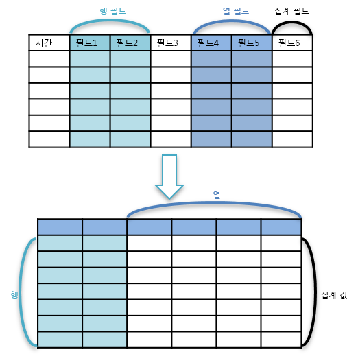
The data analysis process using pivots is as follows:
- Step 1: Data Loading
-
It is more appropriate to consider Data Source Type as the data source to be imported. You can select data source type, time range, target, schema, fields, etc. to import data. In addition, you can use a low-level approach by directly entering a query, or import a pivot file exported externally.
-
For usage by data type, refer to Data Loading.
- Step 2: Data Processing
-
After executing step 1, the work panel switches to a set of tools for full-scale pivot operations, and the imported data is displayed in the workspace.
-
The imported data needs to be processed to make it suitable for analysis. Processing is largely divided into preprocessing and postprocessing. The processing performed in step 2 refers to preprocessing, which involves rearranging and sorting data based on conditions. Rearrangement and sorting are explained in Data Processing.
- Step 3: Data Analysis
-
Define matrices (row/column fields, value fields) to summarize relationships between selected items, aggregate data, or perform correlation analysis with other data to transform it into meaningful forms.
-
In the Data Analysis step, you can also use filters for postprocessing. Steps 2 and 3 are only distinguished for convenience; in practice, they are performed simultaneously.
- Step 4: Utilizing Analysis Results
-
The derived data can be saved as a dataset or configured as a dashboard widget for reuse and visualization.
From here, each task that can be performed in each step will be introduced.
Data Loading
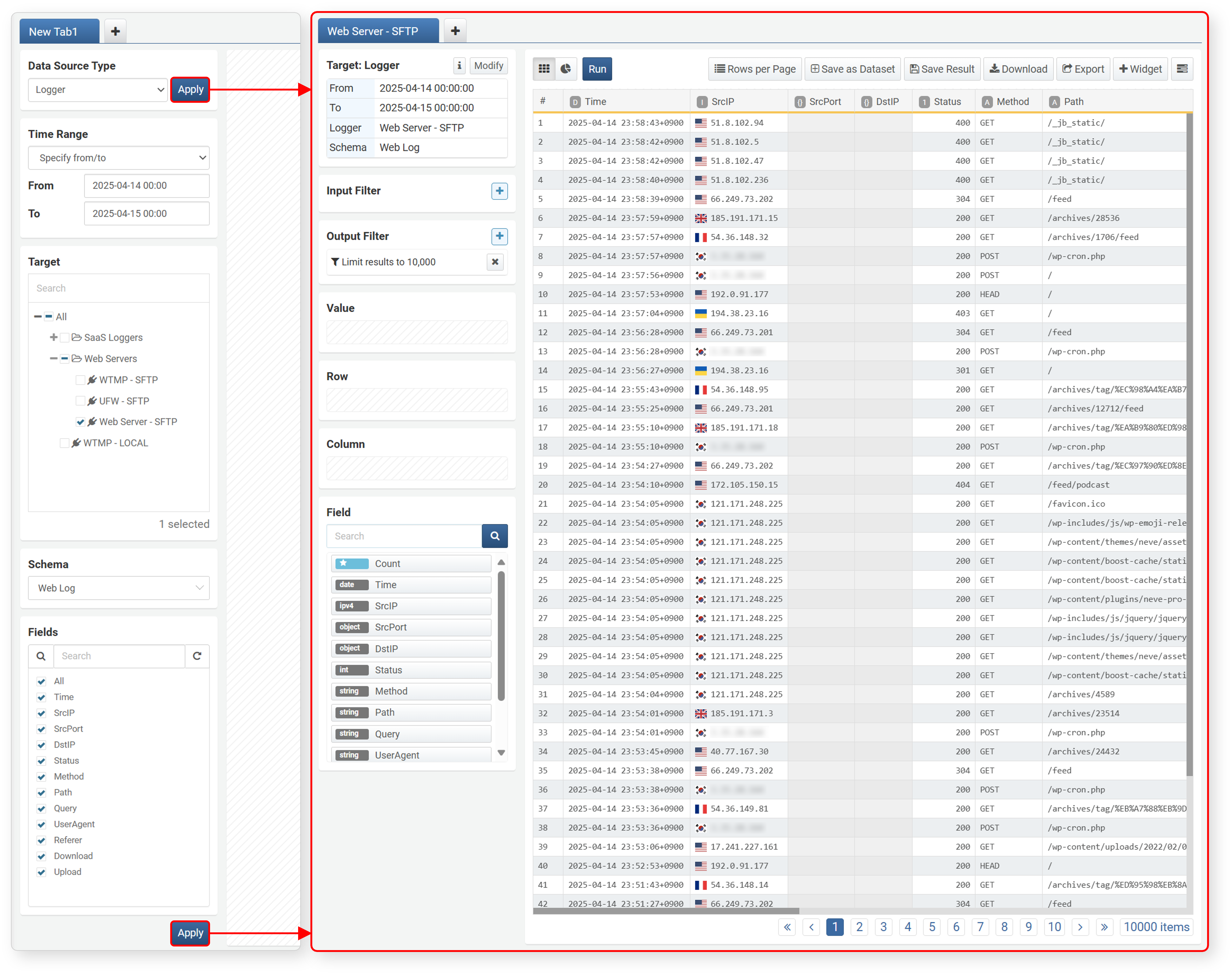
Specify the conditions for data to be imported, such as Data Source Type, Time Range, Target, Schema, and Fields, then click Apply to load the data and display it in the workspace. Up to 10,000 records can be loaded (this can be changed in the result filter).
Data Source Type
Select the type of data to import in the data type section (default: Logger). The list of targets will be shown according to the selected type.
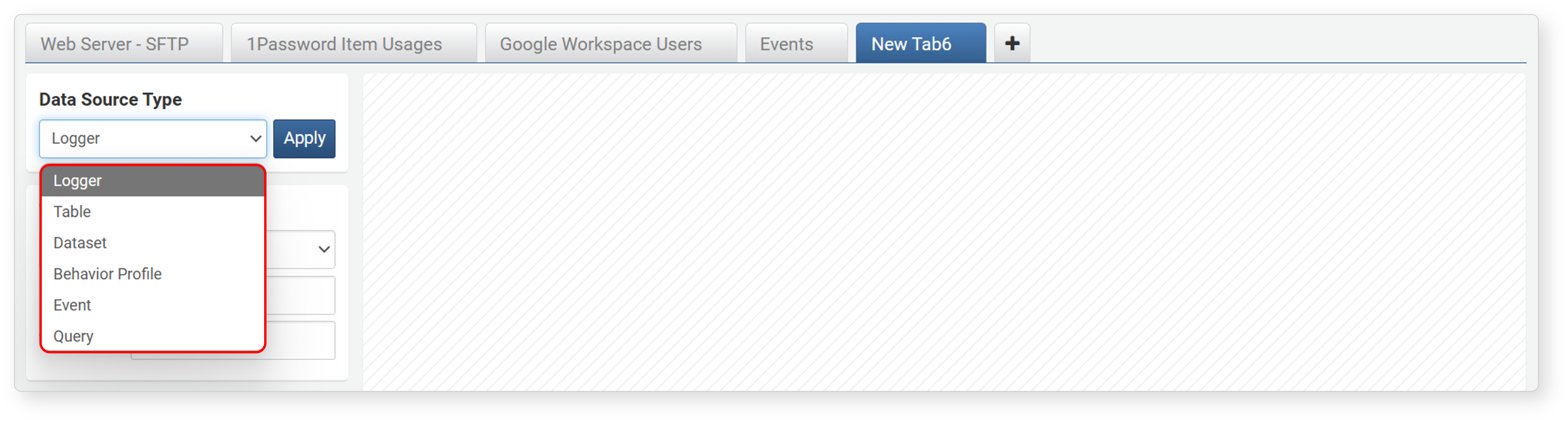
- Logger: Imports data from tables defined in the selected logger. Even if multiple loggers share a table, only data collected by the selected logger will be imported.
- Table: Imports data stored in the selected table.
- Dataset: Imports data by executing a query according to the selected dataset. Since the dataset query has a specified search period and retrieves results based on the execution time, you cannot specify the time range in the data loading settings.
- Behavior Profile: Imports the most recently built data from the selected behavior profile. Using behavior profiles for correlation analysis can be effective for detecting security anomalies.
- Event: Imports event data generated by stream rules or batch rules.
- Query: Imports the result of executing a query entered in Query. If you want to import data not defined by a preset data type, select Query.
Time Range
Range is the setting for the period during which the data occurred (except when the data type is Dataset or Query). This period is applied to the _time field of the data.
The default is the past 24 hours from the current time. However, if the Data Source Type is Behavior Profile, the default is All Time.
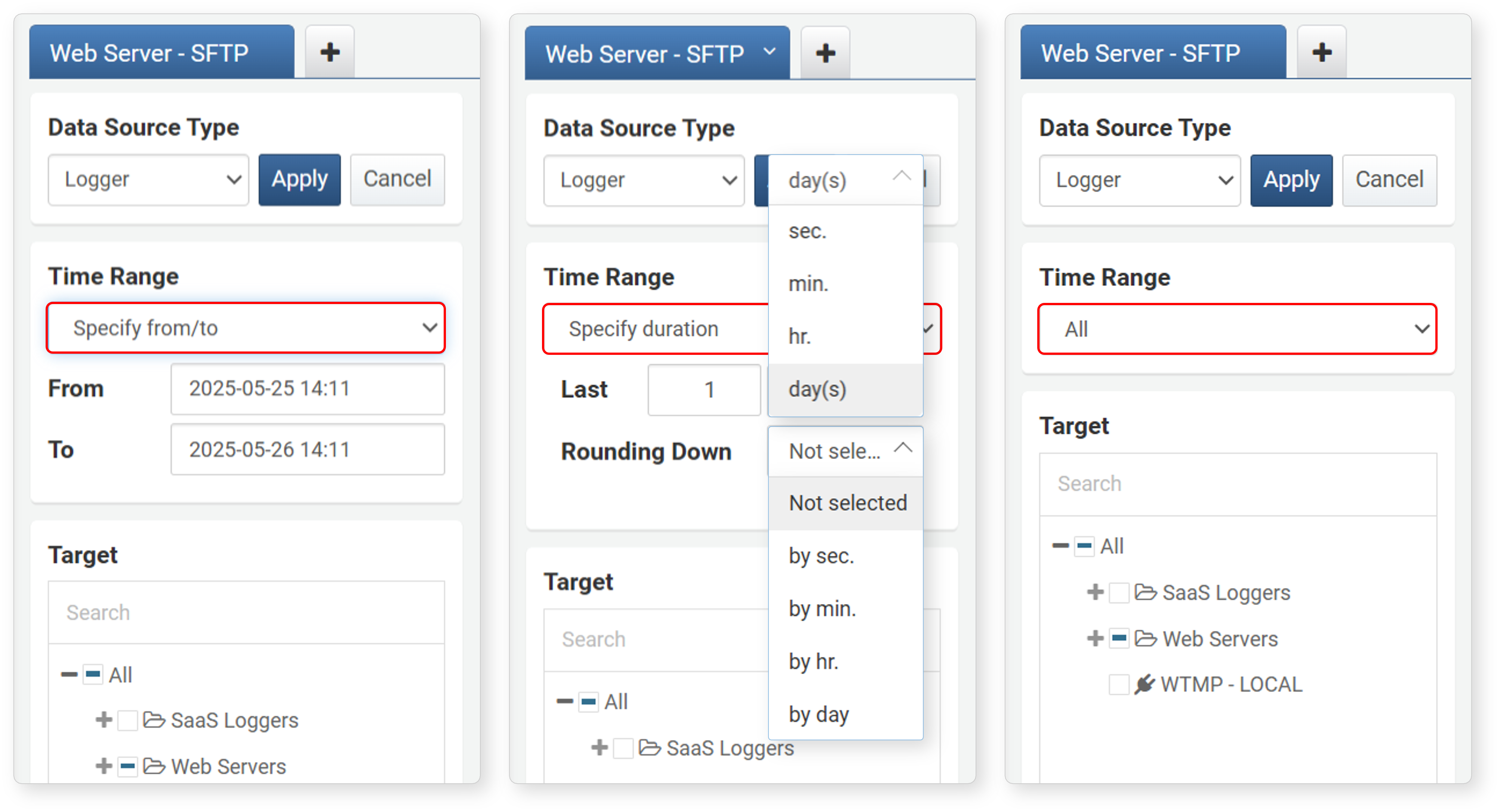
- Specify from/to: Data collected between the specified start (
from) and end (to) times (default: past 24 hours from the current time). The time specified as end is not included in the search range. - Specify duration: Data collected from the specified Last time (
from) up to now (default: 1 day).- Rounding Down (default: Not selected): If you specify a unit (seconds, minutes, hours, days), the _time field values are truncated to that unit (same as applying the datetrunc() function).
- All: Retrieves all data recorded in the target.
Target
When you select a data type, a list is shown according to the selected type. Select one or more targets to query from the list. The following image shows examples of targets by data type.
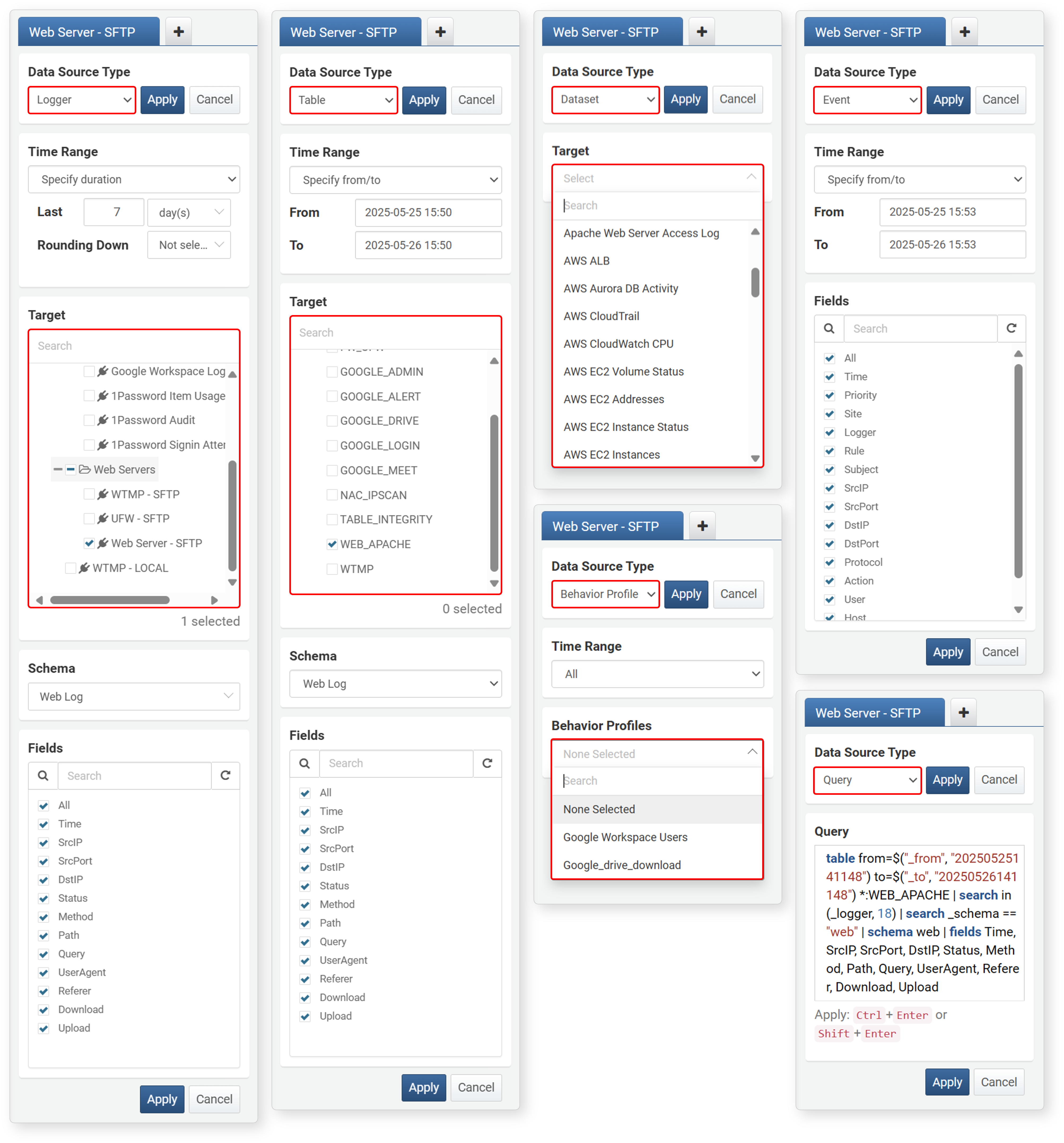
- If the Data Source Type is Behavior Profile, this is shown as Behavior Profiles instead of Target.
- If the Data Source Type is Event or Query, you cannot use Target.t
If you need to apply different log schemas, open a new tab for each and then try correlation analysis.
Schema
Schema can be specified when the data type is Logger or Table. Specifying a schema normalizes the original fields of the data to the field names defined in the schema. Fields not defined in the schema are not imported.
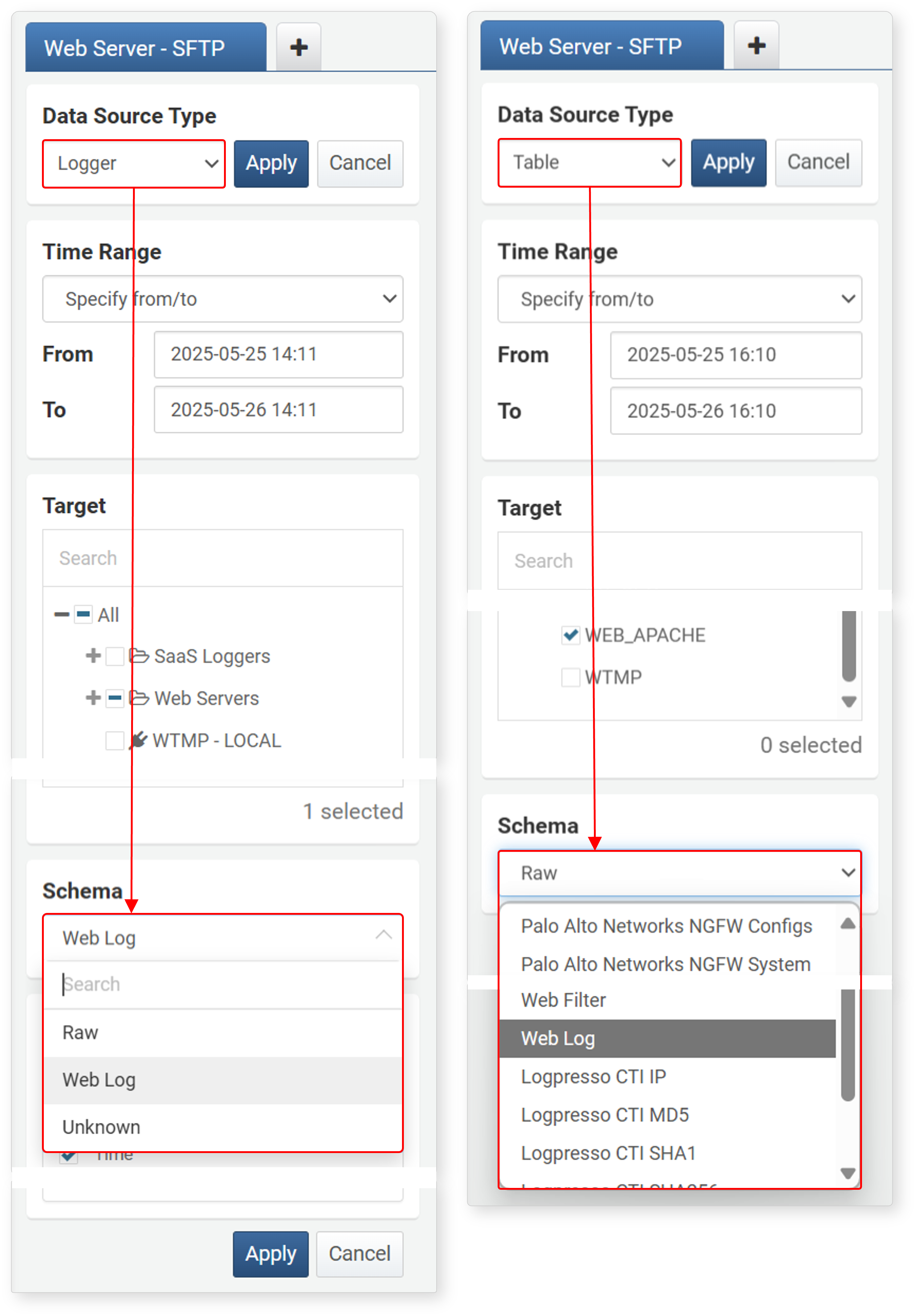
- If the Data Source Type is Logger, you can select from the log schemas defined in the logger model's normalization rules, as well as Raw and Unknown.
- If the Data Source Type is Table, since there is no separate schema information linked to the table, you can select from all log schemas (including Raw and Unknown). Check which log schema was applied when recording data to the table, then select the log schema.
- Unknown is used to display unknown data that does not match any normalization rule in the logger model.
- If you want to import the original fields without normalization, select Raw in the schema list.
Fields
Fields are shown according to the schema selected when the Data Source Type is Logger, Table, or Event.
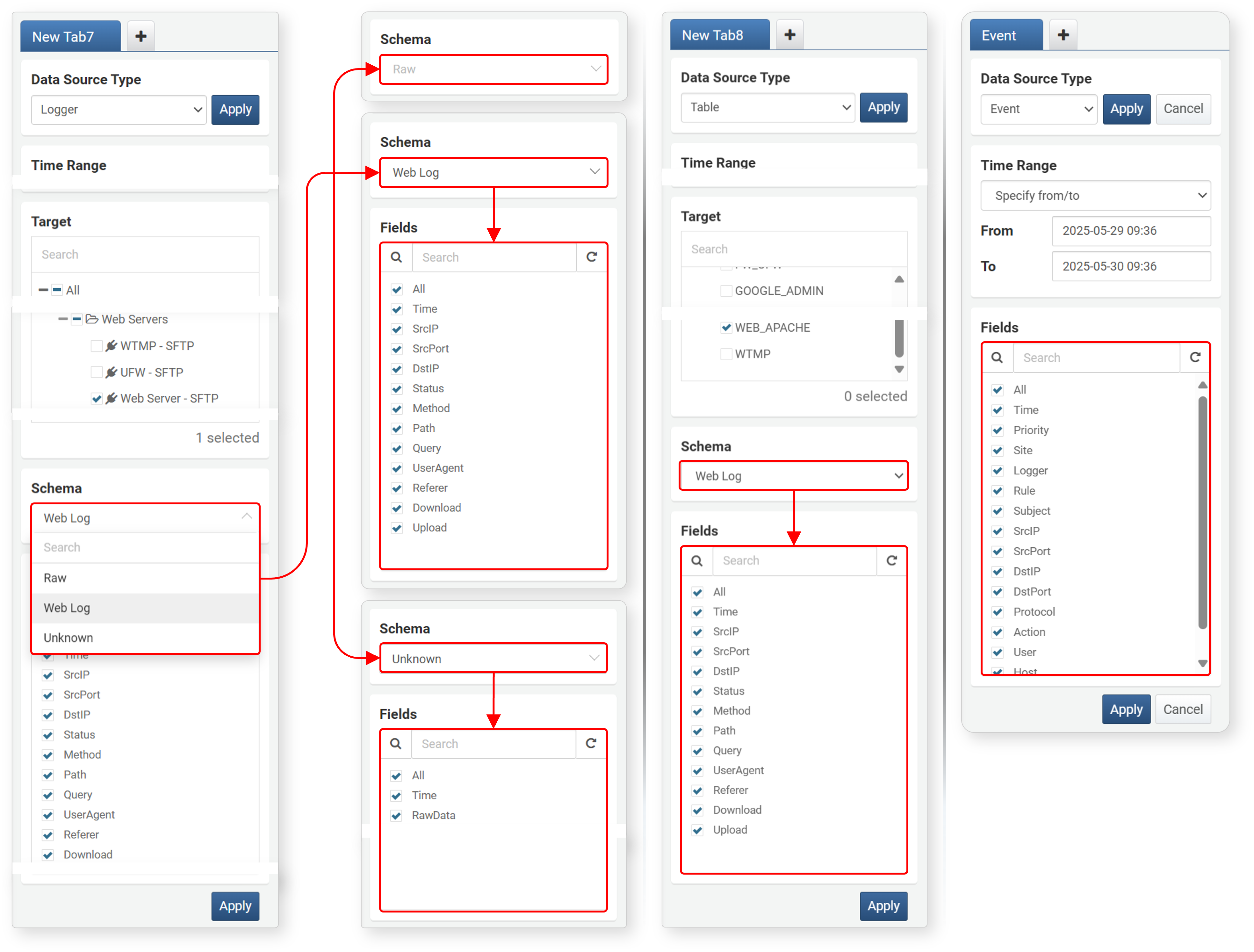
- If Raw is selected in Schema, no field list is provided since normalization is not applied.
- If the Data Source Type is Event, the event normalization field list is shown without schema selection.
- Deselect unnecessary items from the field list.
Query
When the data type is Query, a query input box appears.
- The query input box supports auto-completion and query execution shortcuts.
- All settings such as data search period and field list must be specified directly in the query.
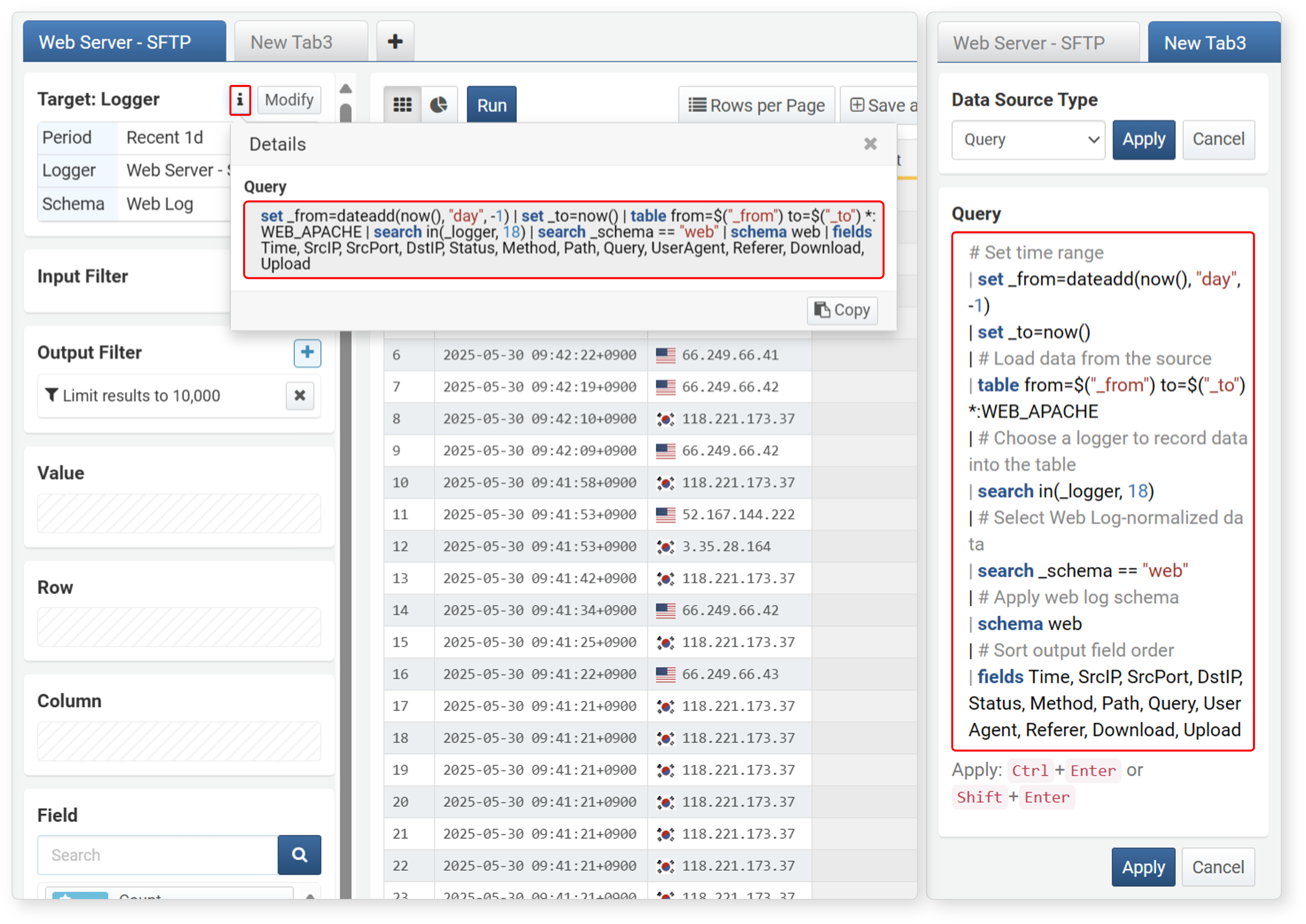
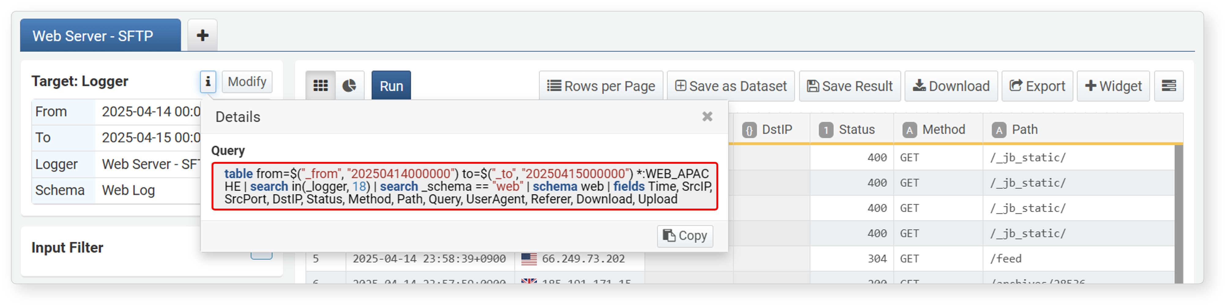
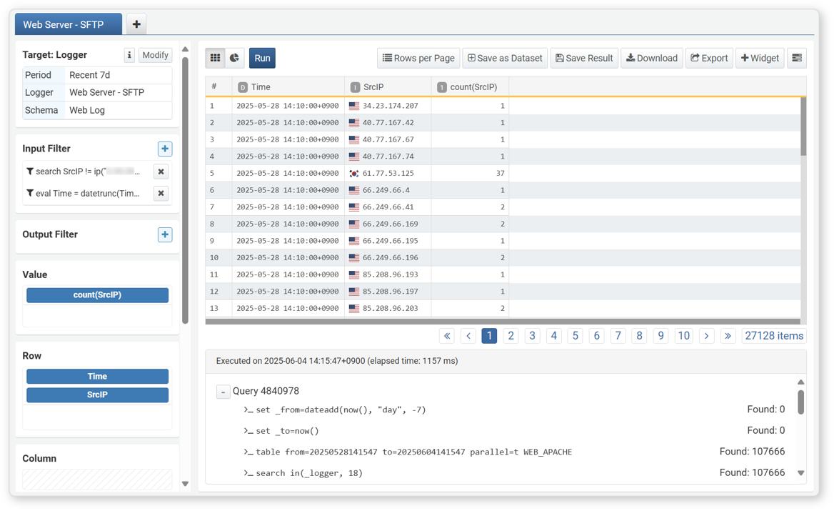
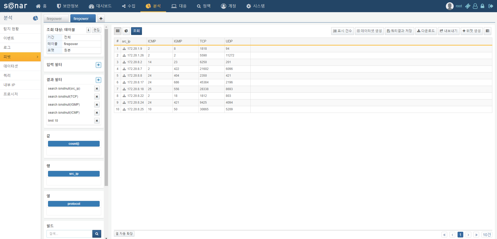
The following image shows an example of configuring data import from a logger using a query. The left shows data imported by selecting Logger as the data type, and the right shows data imported by entering a query after selecting Query as the data type.
-
Click
 to check the query applied when importing data. Both import settings provide the same functionality.
 -
The entered query is as follows:
# Data search period
| set _from=dateadd(now(), "day", -1) | set _to=now()
| # Select table to import data from
| table from=$("_from") to=$("_to") *:WEB_APACHE
| # Select logger that recorded data to the table
| search in(_logger, 1)
| # Select data with normalization rule 'web log'
| search _schema == "web"
| # Apply web log schema
| schema web
| # Arrange output field order
| fields Time, SrcIP, SrcPort, DstIP, Status, Method, Path, Query, UserAgent, Referrer, Download, Upload
Load
Click Apply to load data into the workspace according to the specified data type, range, target, schema, and fields, and the work panel will change to suit data processing and pivot operations.
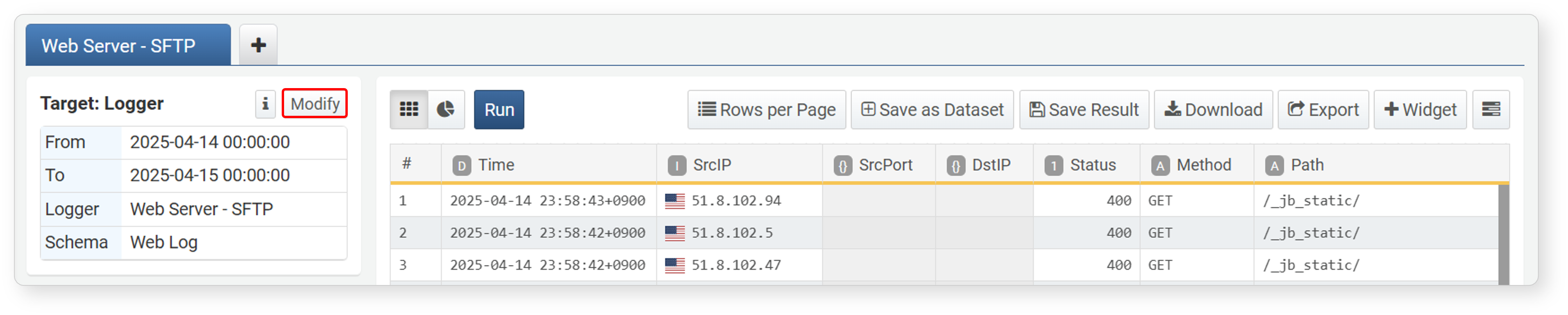
Reload
To reload data with different conditions, click Edit next to Target in the work panel, modify the conditions, and then click Apply.
View Query
Click the icon next to Target in the upper left to check the data search query. Click Copy to copy the query to the clipboard.
Data Processing
Once data is loaded, it is displayed in the workspace. Process the data into a form suitable for aggregation or analysis. Remove unnecessary data, truncate the time unit according to the analysis period, sort it into an analysis-friendly format, and select only the required data to facilitate pivot operations.
Logpresso Sonar provides three categories of features: filters, expressions, and sorting.
- Filter: A tool for retrieving only data that matches specific conditions, or for selecting only data that meets certain criteria from data processed through a pivot.
- Expression: Used to truncate imported date data by time unit, calculate time differences, or convert strings.
- Sort: Tools for rearranging data (e.g., changing column order, hiding columns, ascending/descending order, top/bottom N) and changing display formats (cell data alignment).
How to Use
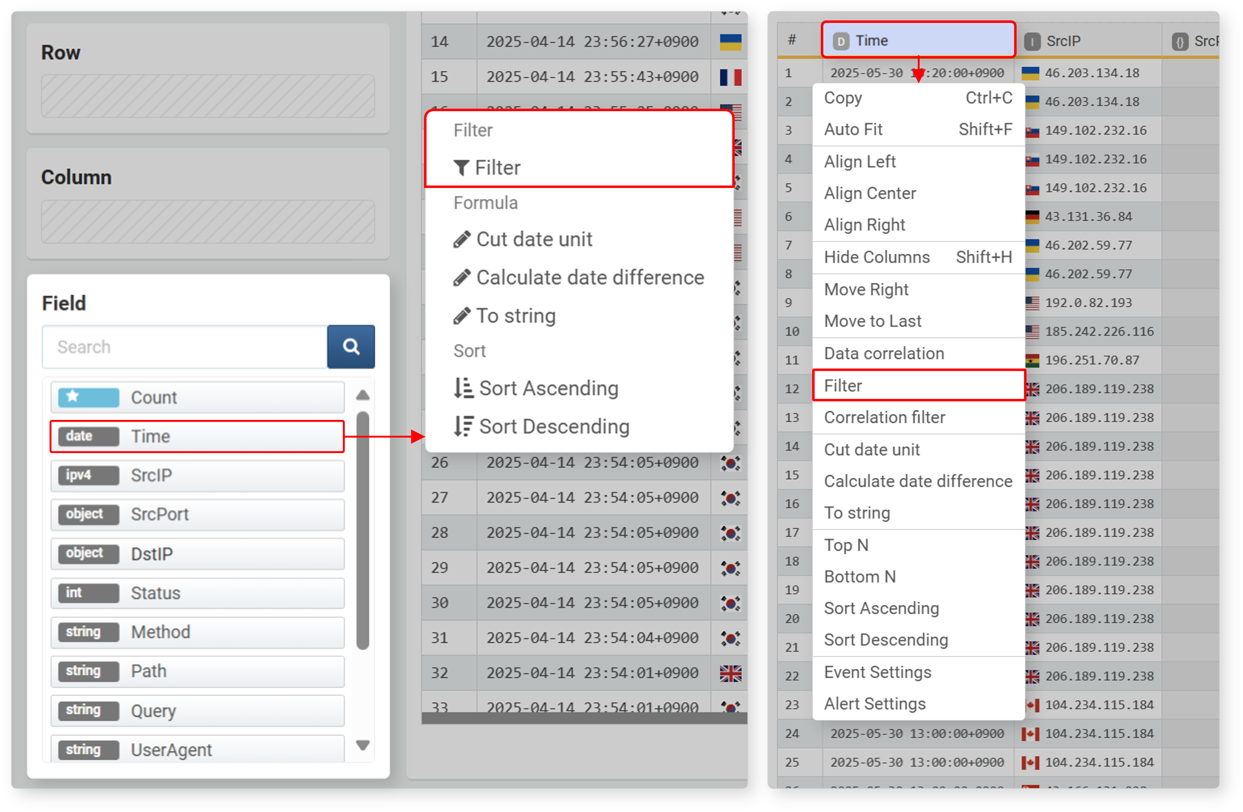
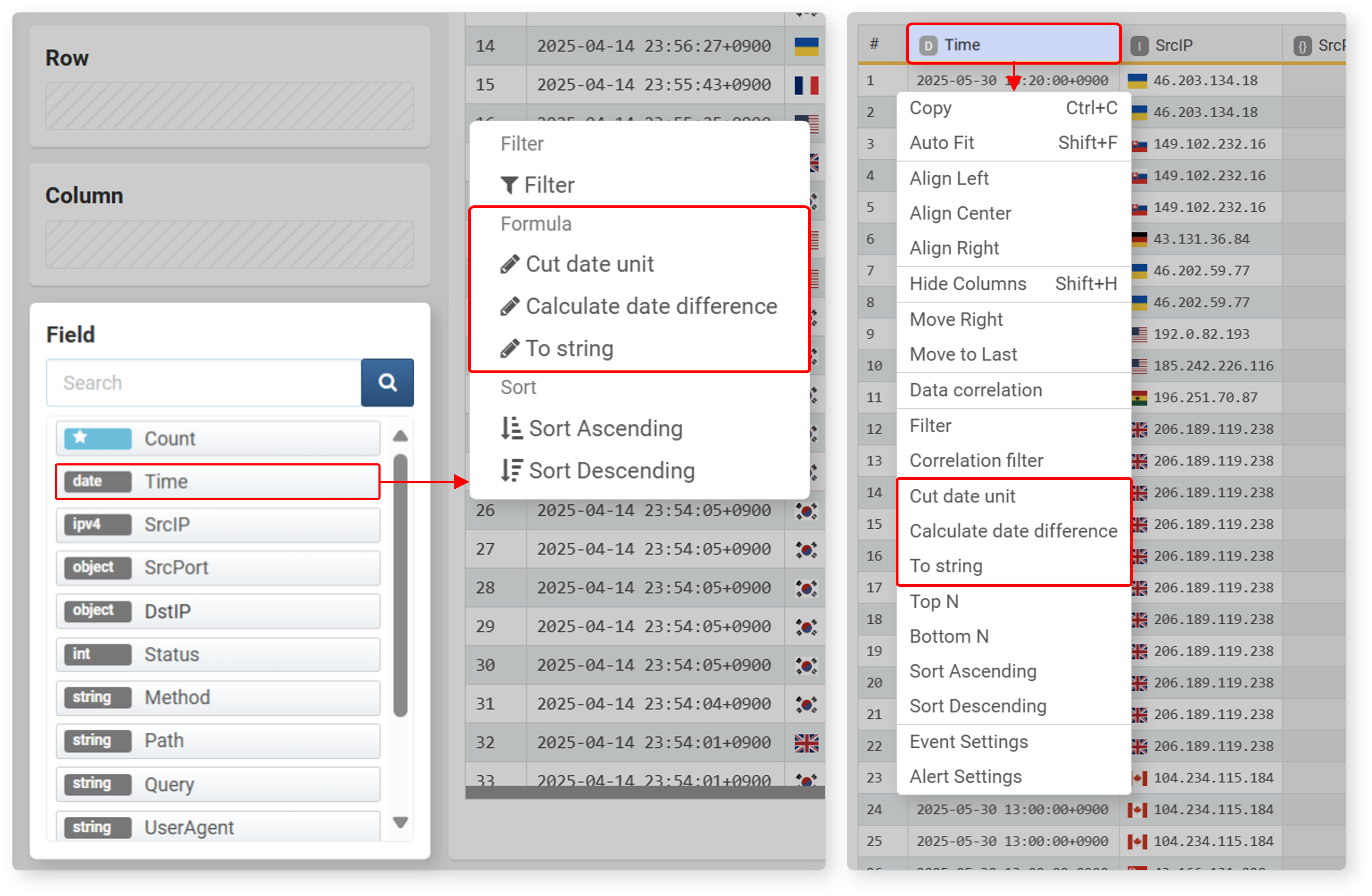
Filter, expression, and sort functions are available from the field list, column (field name) in the pivot table, and cells in the pivot table.
- Click a field in the field list
- In the data loading settings area, select and click a field from the field list to use filter, expression, and sort functions.
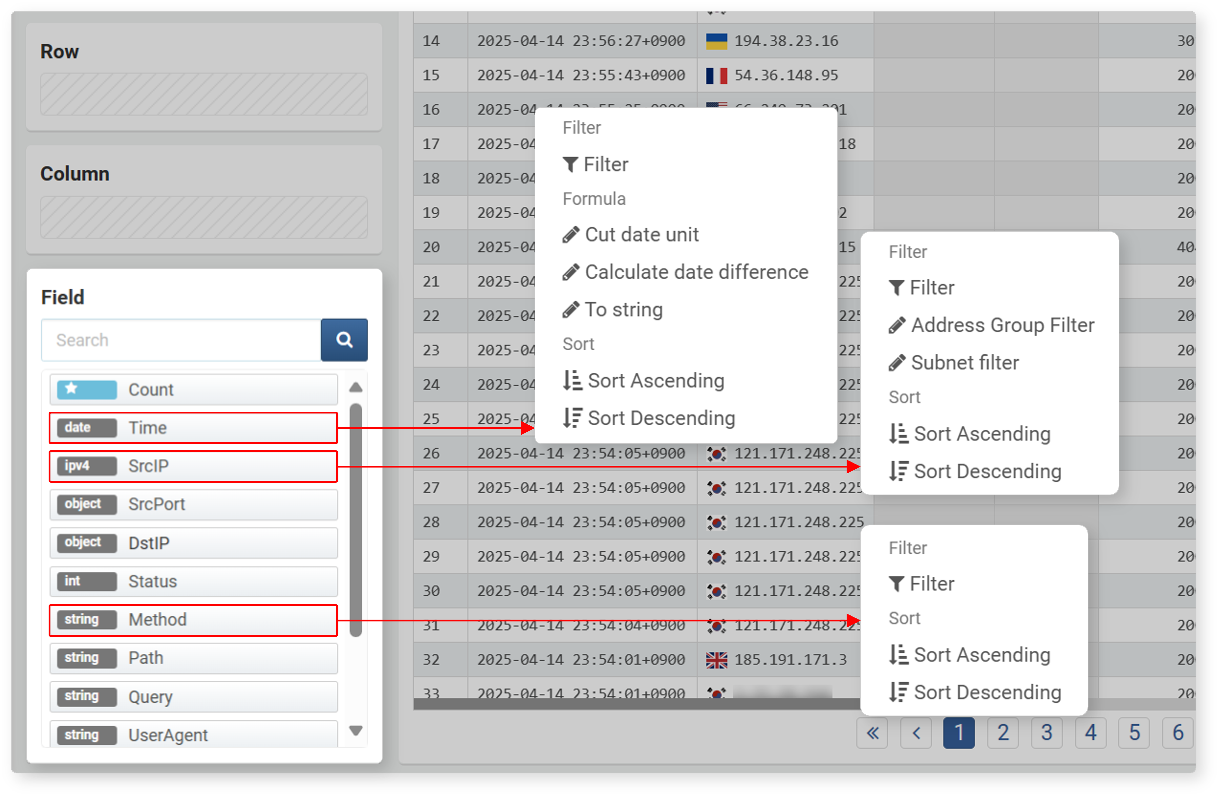
- The filter/expression/sort is applied based on the data column matching the selected field.
- The data type of each field is displayed to the left of the field.
- Available filters may vary depending on the data type.
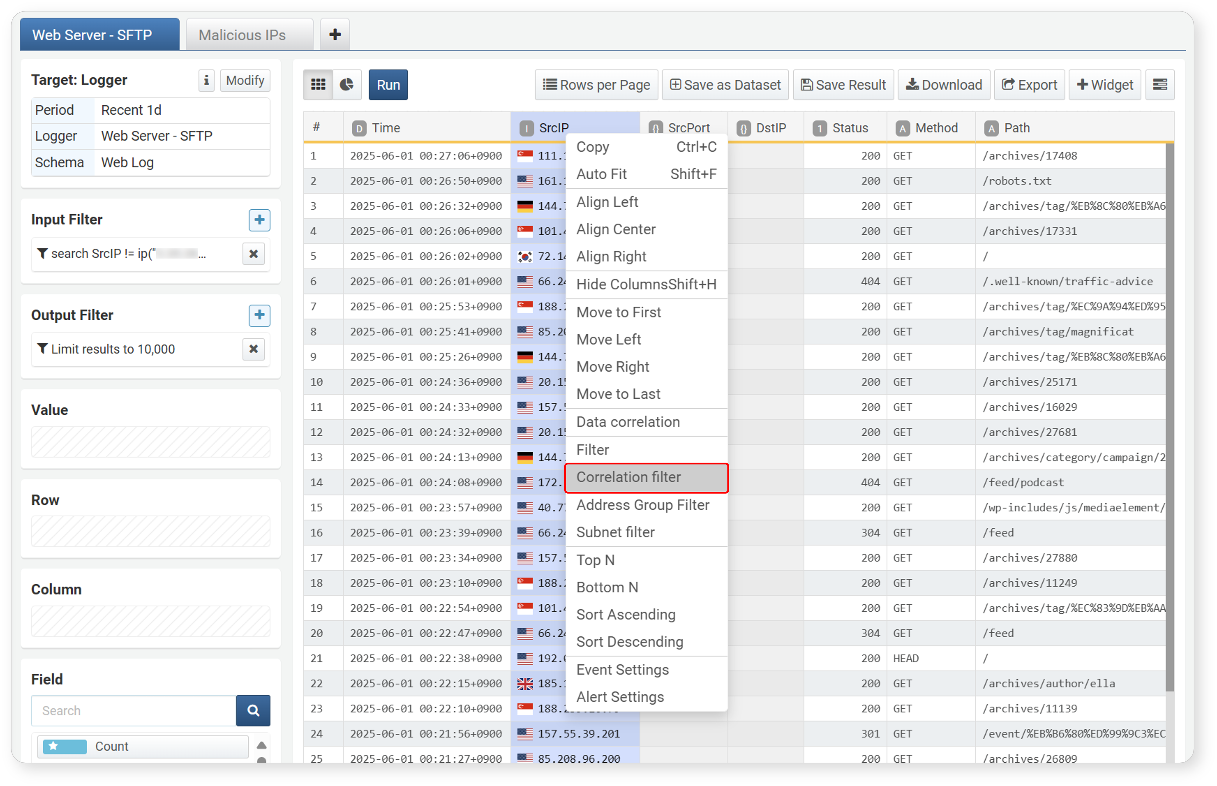
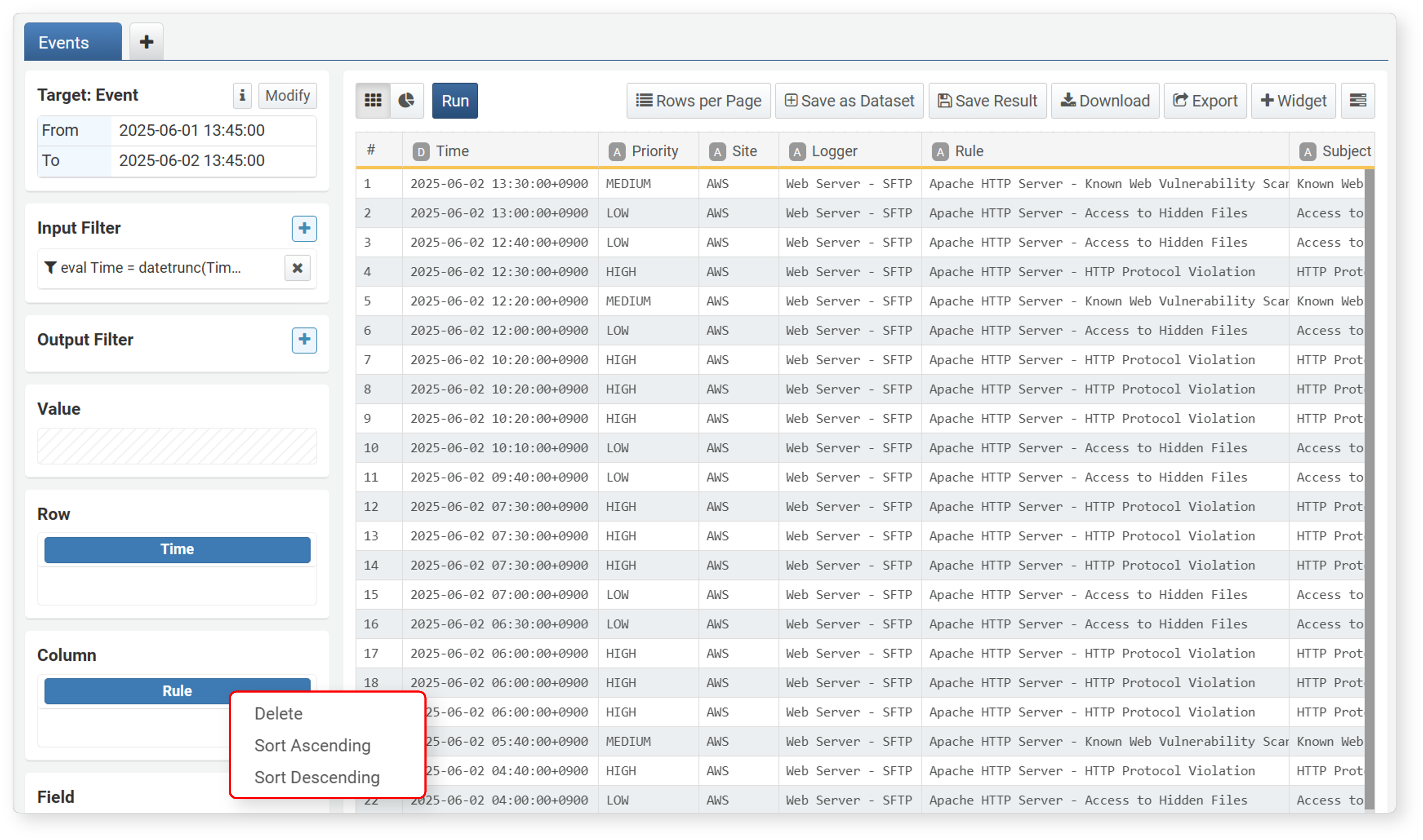
- Right-click a column name
- In the workspace, right-click (usually the right mouse button) the data column name (field) to use these functions. You can move columns, sort ascending/descending, select top/bottom N, etc.
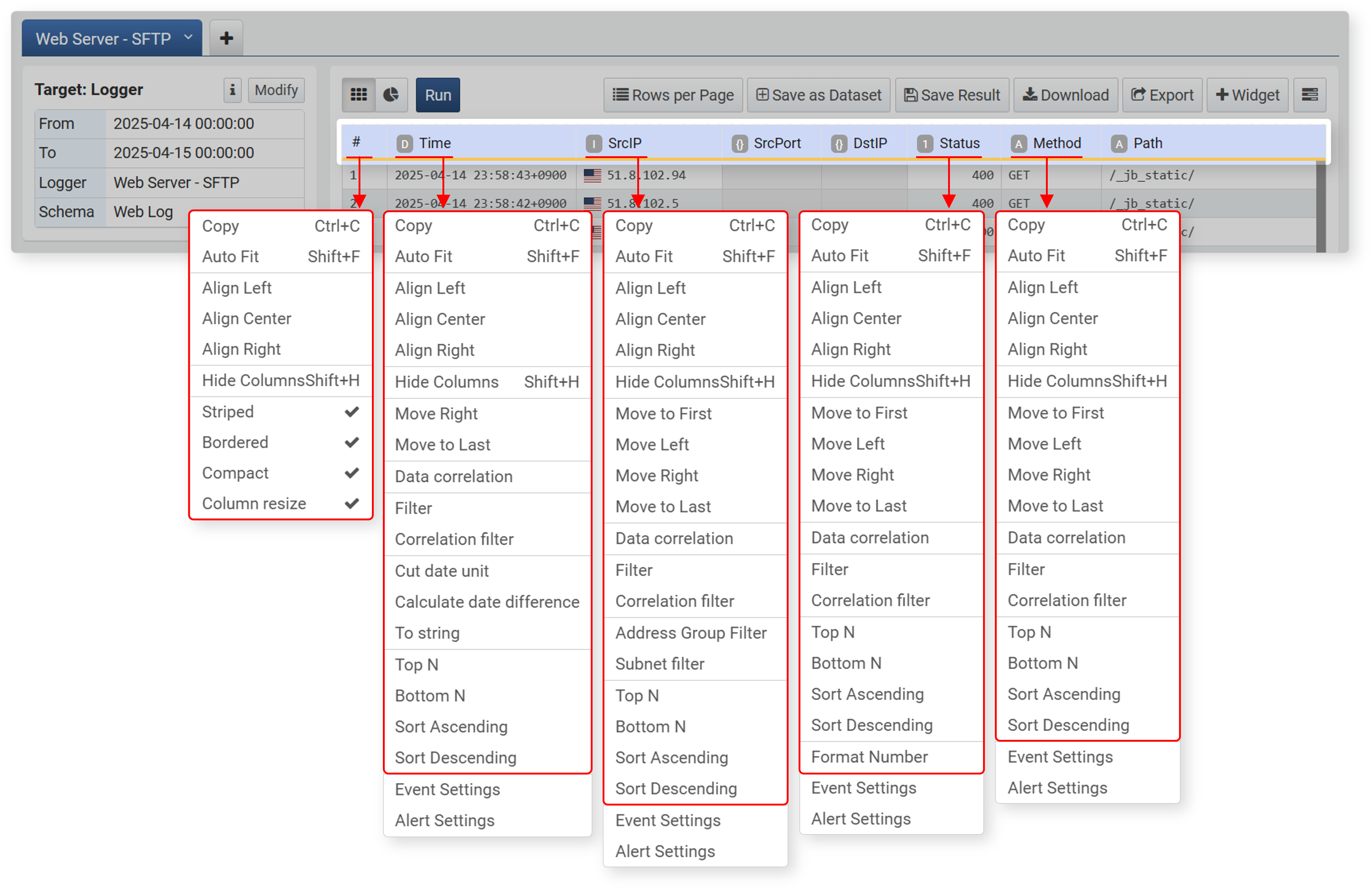
- You can specify the position of data columns and sorting within columns, which cannot be defined in the field list.
- Provides hide/unhide column functions. Hidden columns are indicated by a bold solid line.
- Right-clicking the # (row number) column selects the entire column and allows you to change the style of the data grid.
- When there are multiple pivot tabs, you can perform correlation analysis between two pivot tables.
- Besides correlation analysis, you can use correlation filters.
- Event and alert settings are used when configuring widgets.
- Right-click a cell
- In the workspace, right-click (usually the right mouse button) a specific cell to apply a filter based on the cell value.
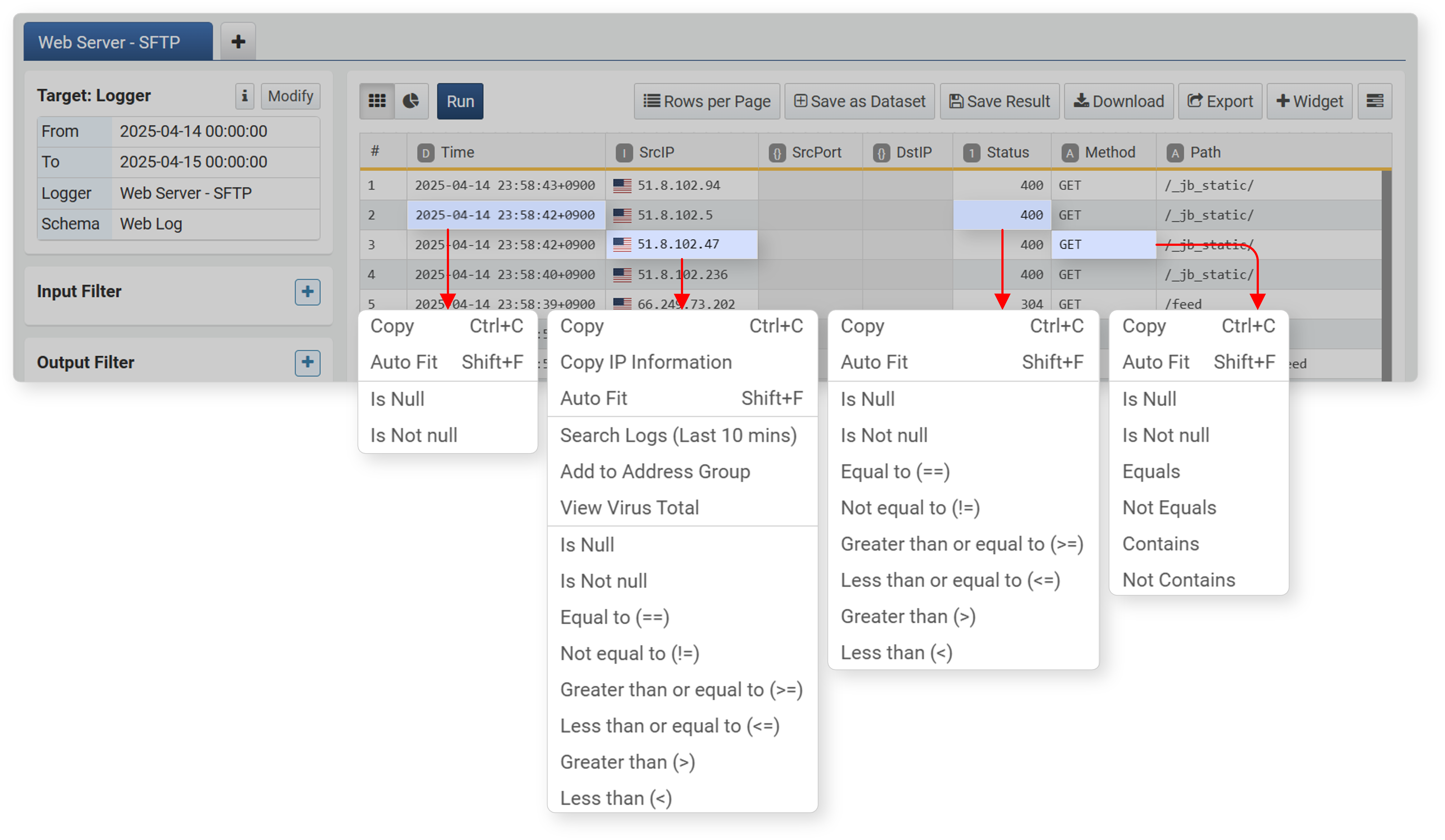
- You can apply filters based on cell data. Available filters may vary depending on the data type.
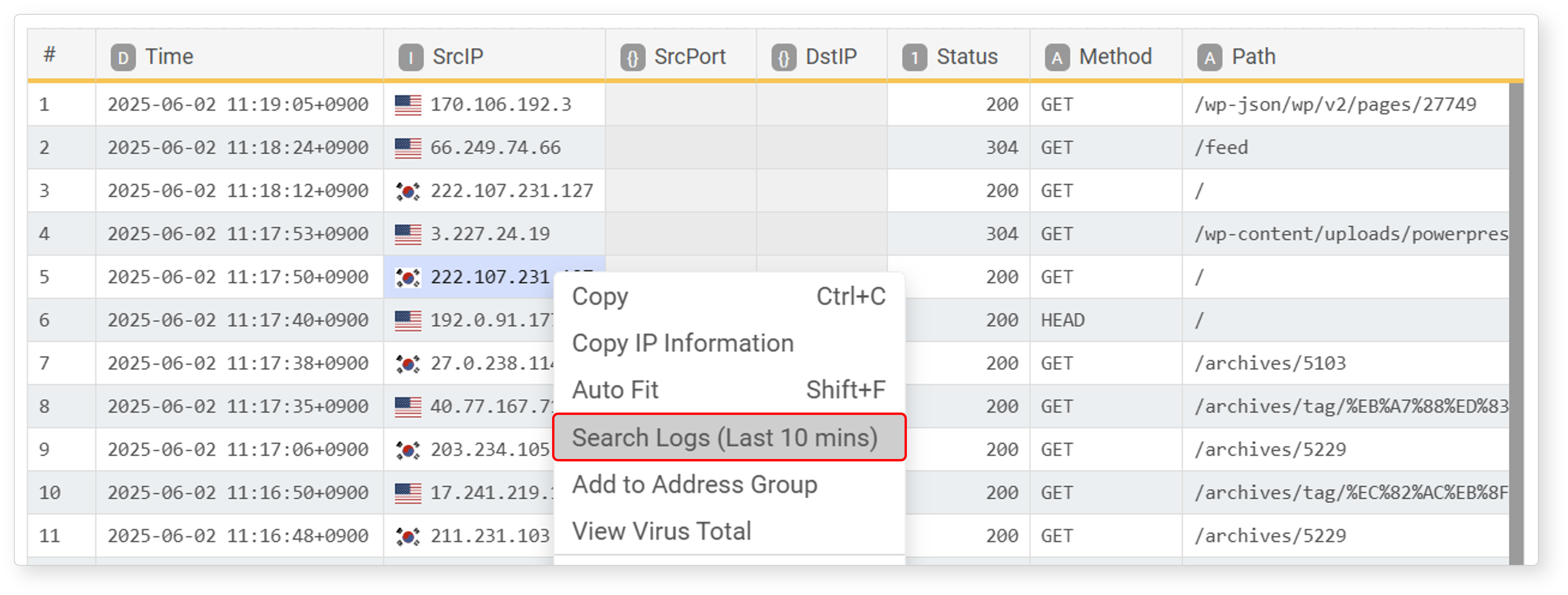
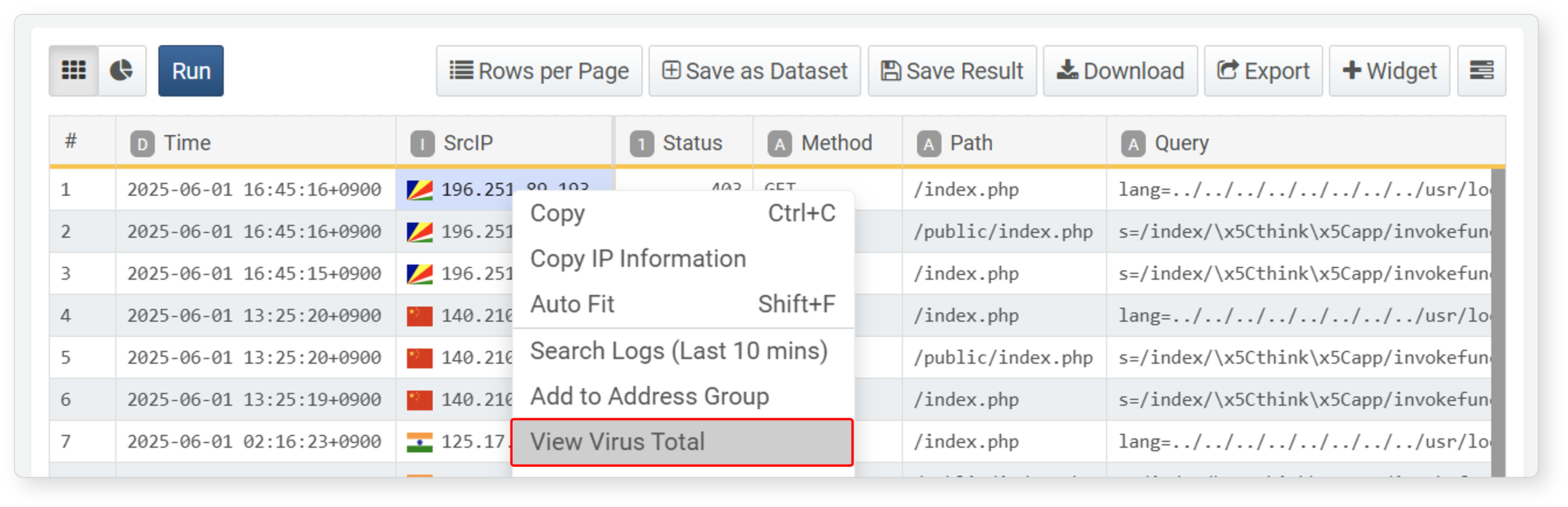
- When selecting IP address data, Search Logs (Last 10 mins), Add to Address Group, and View VirusTotal functions are provided.
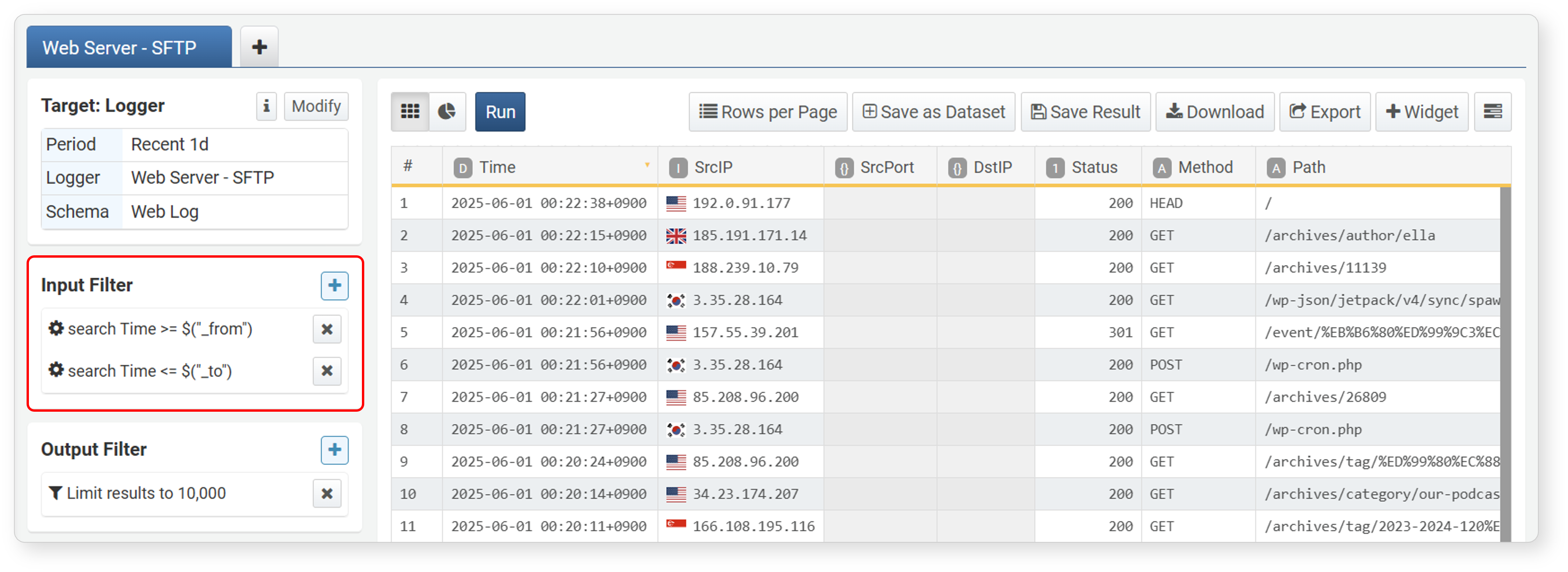
Input/Result Filters
Filters, expressions, and sorting are all converted into queries and applied. Filters/expressions/sorting applied during data loading are shown in the input filter, and those applied to analysis results are shown in the result filter.
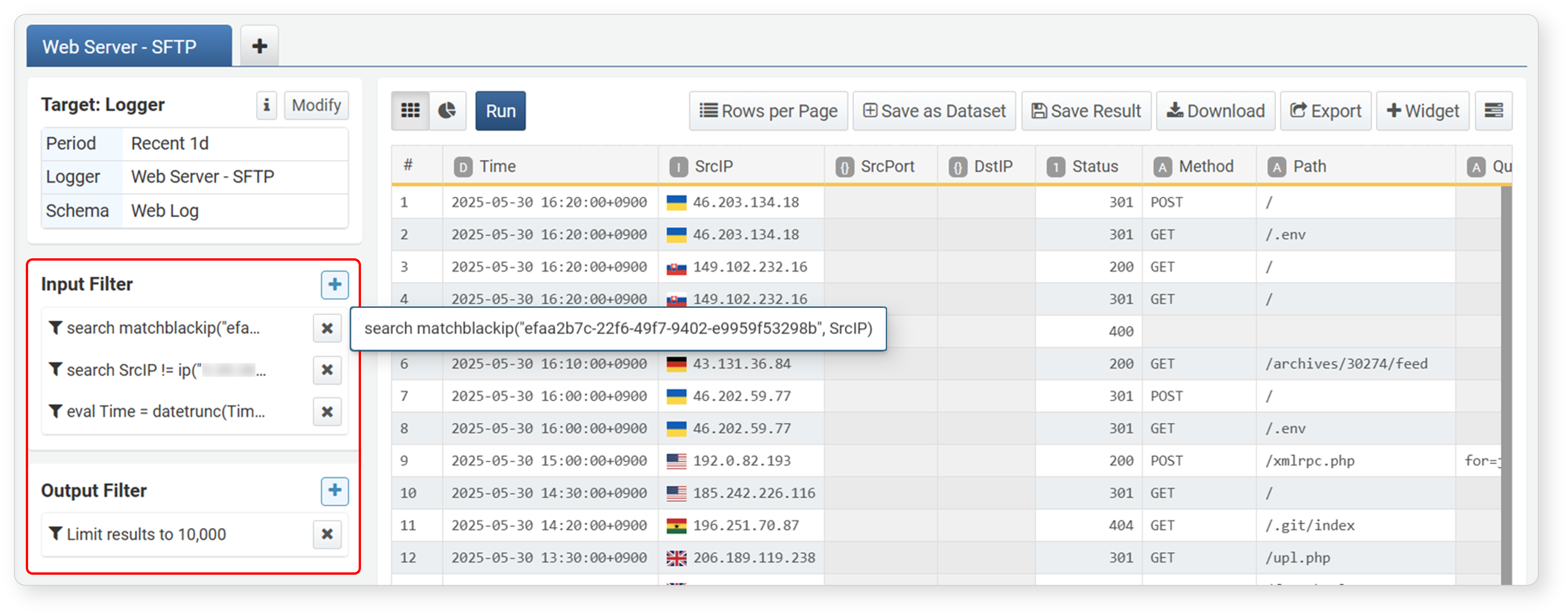
- Input Filter: If you apply a filter/expression/sort before setting aggregation values, it acts as an input filter. Filter queries are executed as input for the query results shown in View Query.
- Result Filter: In the Data Analysis stage, filters/expressions/sorting are applied to the aggregated data after rows, columns, and values are set.
A query with a funnel icon indicates a filter. A query with a gear icon indicates a filter containing a user-defined variable.
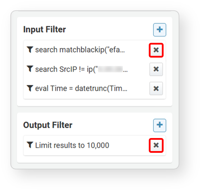
Removing Filters
To remove an applied filter, click  to the right of the filter in the input or output filter section.
Filter
Filters are used to retrieve only data that matches specific conditions or to select only data that meets certain criteria from data processed through a pivot.
Filter Conditions
Filter conditions are used when you want to select only data with field values that meet specified criteria. To apply a filter condition, click Filter in the field popup menu or Filter Condition in the column name popup menu.
You can specify search conditions in the Add Filter dialog.
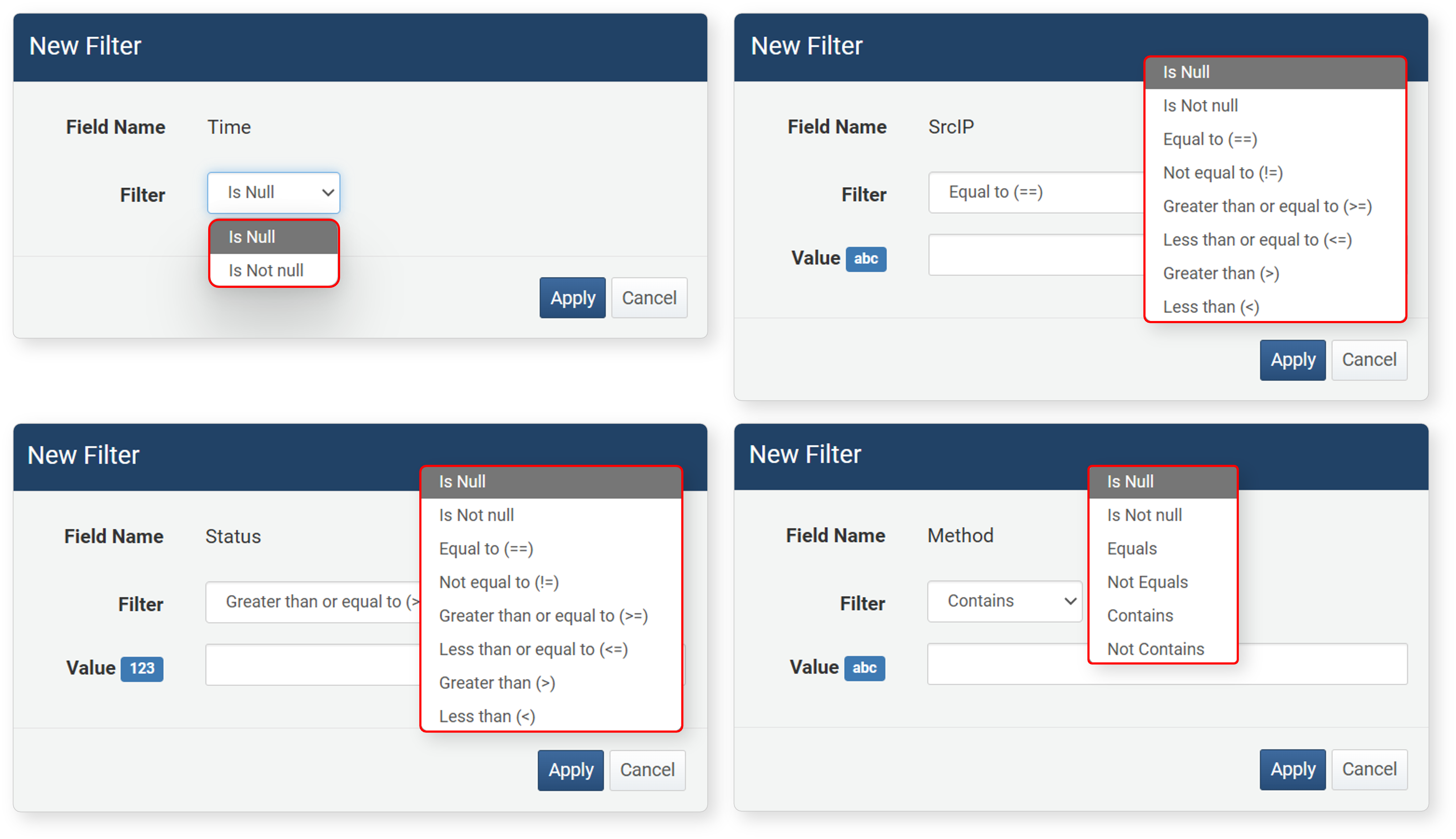
- Field Name: The field (column name) to apply the filter to
- Filter: Comparison condition. The available conditions depend on the data type of the field.
- Value: The value to compare against
You can also set a filter directly from the cell popup menu by selecting a comparison condition. In this case, the cell value is used as the comparison value.
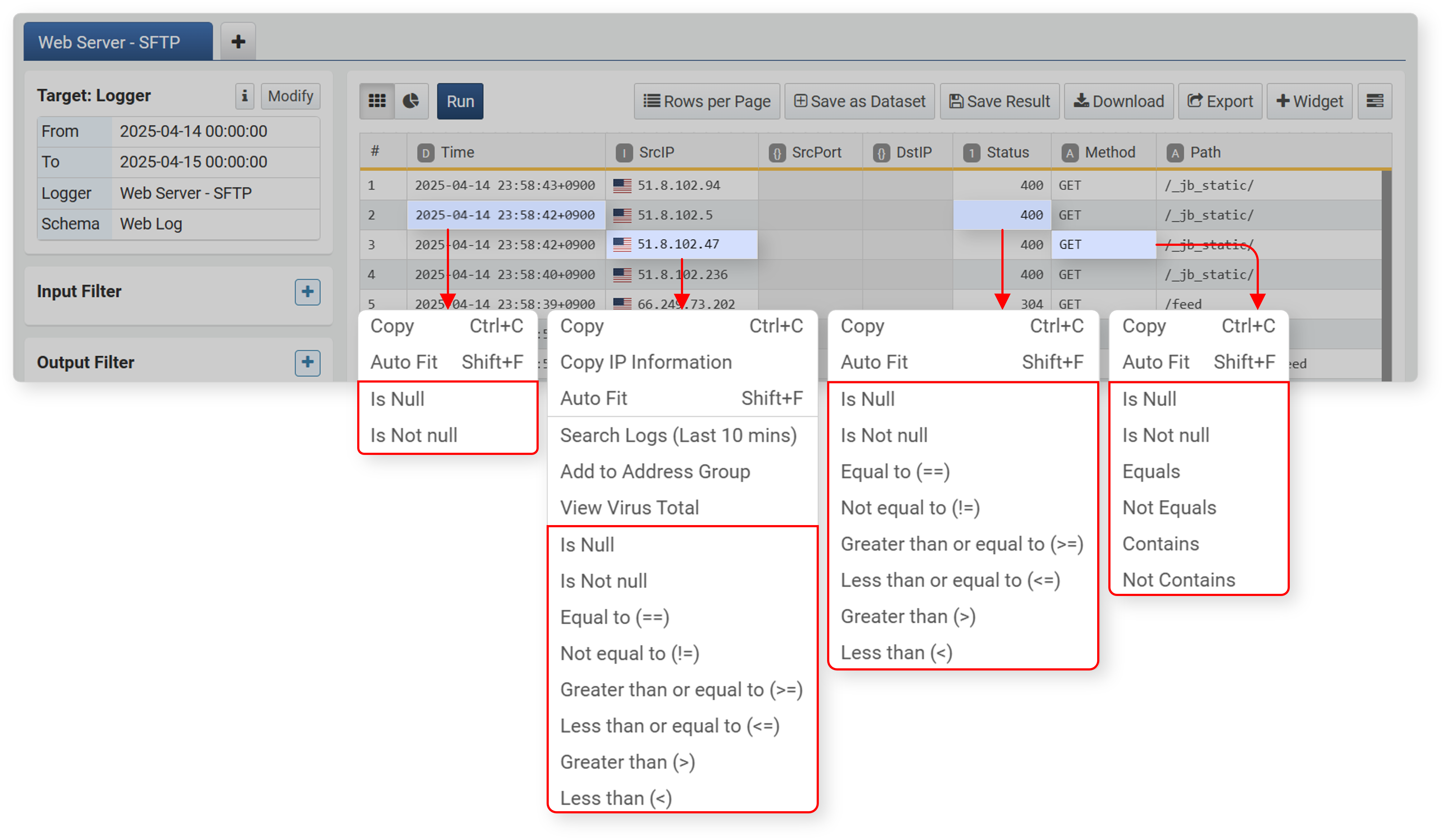
Below are the available comparison conditions by data type. The set filter is converted into a query and registered in the input filter or output filter.
| Condition | Data Type | Query |
|---|---|---|
| Is Null | All types (including list, object) | search isnull(FIELD_NAME) |
| Is Not Null | All types (including list, object) | search isnotnull(FIELD_NAME) |
| Equals (==) | IP address, integer, float | search FIELD_NAME == VALUE_EXPR |
| Not Equals (!=) | IP address, integer, float | search FIELD_NAME != VALUE_EXPR |
| Greater or Equal (>=) | IP address, integer, float | search FIELD_NAME >= VALUE_EXPR |
| Less or Equal (<=) | IP address, integer, float | search FIELD_NAME <= VALUE_EXPR |
| Greater (>) | IP address, integer, float | search FIELD_NAME > VALUE_EXPR |
| Less (<) | IP address, integer, float | search FIELD_NAME < VALUE_EXPR |
| Match | String | search FIELD_NAME == "STR" |
| Not Match | String | search FIELD_NAME != "STR" |
| Contains | String | search contains(FIELD_NAME, "STR") |
| Not Contains | String | search not(contains(FIELD_NAME, "STR")) |
For filtering fields with boolean values (true or false), refer to General Filter (Query Filter).
Address Group Filter
The address group filter is a dedicated filter that can be applied to fields of the IP address type. It is used to retrieve only IP addresses that belong to or do not belong to a specific address group. This allows you to manage IP addresses by group and quickly retrieve data belonging to a specific group.
To set an address group filter, click Address Group Filter in the field or column name popup menu.
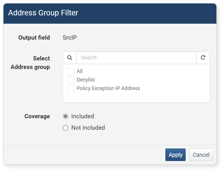
- Output Field: The field (column name) to apply the filter to
- Select Address Group: Select one or more registered address groups
- Coverage: Comparison condition (default: Include)
- Included: Show only values in the output field that are included in the address group
- Not Included: Show only values in the output field that are not included in the address group
The address group filter is converted into the following query and registered in the input/output filter.
| Condition | Query |
|---|---|
| Included | search matchblackip("ADDRGRP_GUID", FIELD_NAME) |
| Not Included | search not(matchblackip("ADDRGRP_GUID", FIELD_NAME) |
If you select two or more address groups, the query is converted to include the "or" logical operator: search not((matchblackip("efaa2b7c-22f6-49f7-9402-e9959f53298b", SourceIP) or matchblackip("c310a9a0-5c04-414a-8b7e-66cd1807c2ab", SourceIP)))
Subnet Filter
The subnet filter is a dedicated filter that can be applied to fields of the IP address type. It is used to retrieve only IP addresses that belong to or do not belong to a specific subnet. This is useful for extracting data for specific ranges according to network structure.
To set a subnet filter, click Subnet Filter in the field or column name popup menu.
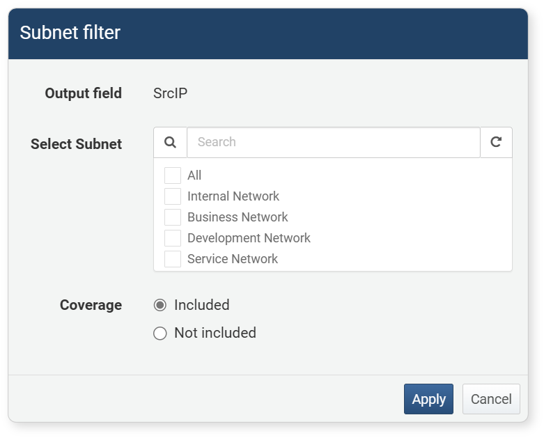
- Output Field: The field (column name) to apply the filter to
- Select Subnet: Select one or more registered subnet
- Coverage: Comparison condition (default: Include)
- Included: Show only values in the output field that are included in the address group
- Not included: Show only values in the output field that are not included in the address group
The subnet filter is converted into the following query and registered in the input/output filter.
| Condition | Query |
|---|---|
| Included | search matchnet("SUBNETGRP_GUID", FIELD_NAME) |
| Not Included | search not(matchnet("SUBNETGRP_GUID", FIELD_NAME)) |
If you select two or more subnets, the query is converted to include the "or" logical operator: search matchnet("bb994ca4-1471-4b91-89f2-99a61bd529b5", SourceIP) or matchnet("bb8525ea-791a-4b8b-94c6-7720da420eb8", SourceIP)
Advanced Filters
Query Filter
You can directly enter a filter query in the input filter or output filter to apply advanced searches not supported by the default filters.
-
In the input filter or output filter, click
 > General Filter.
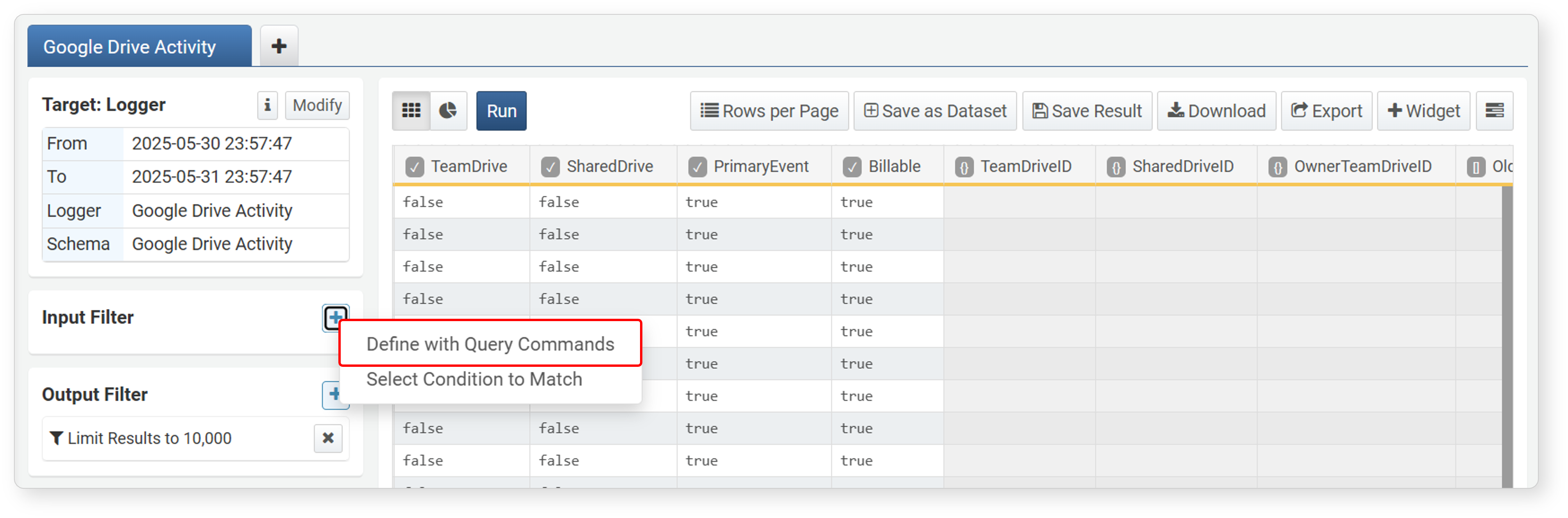
-
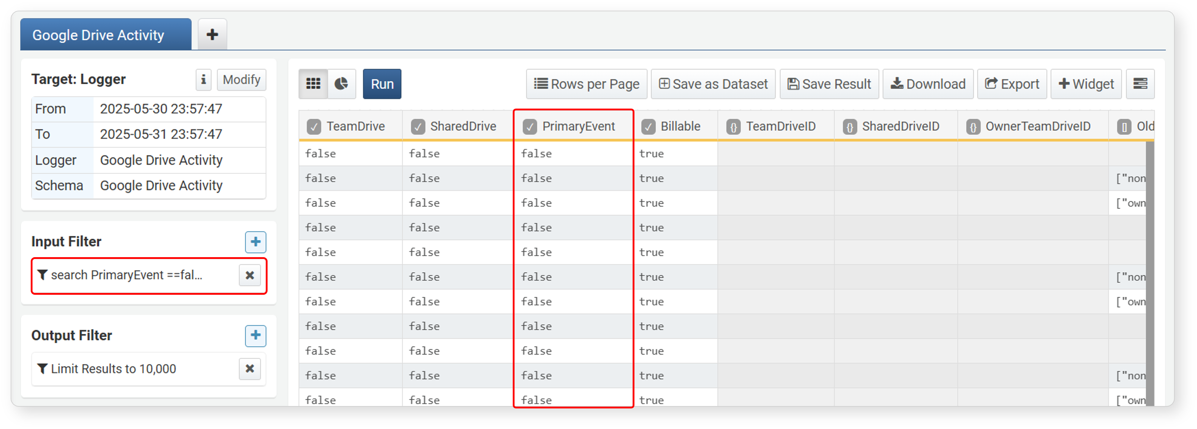
Enter the query to execute in the input filter. For example, to filter records with only
trueorfalsevalues in a boolean field, enter a filter query likesearch FIELD_NAME == trueorsearch FIELD_NAME == falseand click Add.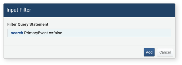
-
Check the results after the filter is applied.
Dynamic Filter
A dynamic filter is used when utilizing analyzed data as a dashboard widget and applying user input from an input control widget to data search.
For a dynamic filter to work, the input control widget and the dynamic filter must use the same user input variable.
-
In the input filter or output filter, click
> Dynamic Filter.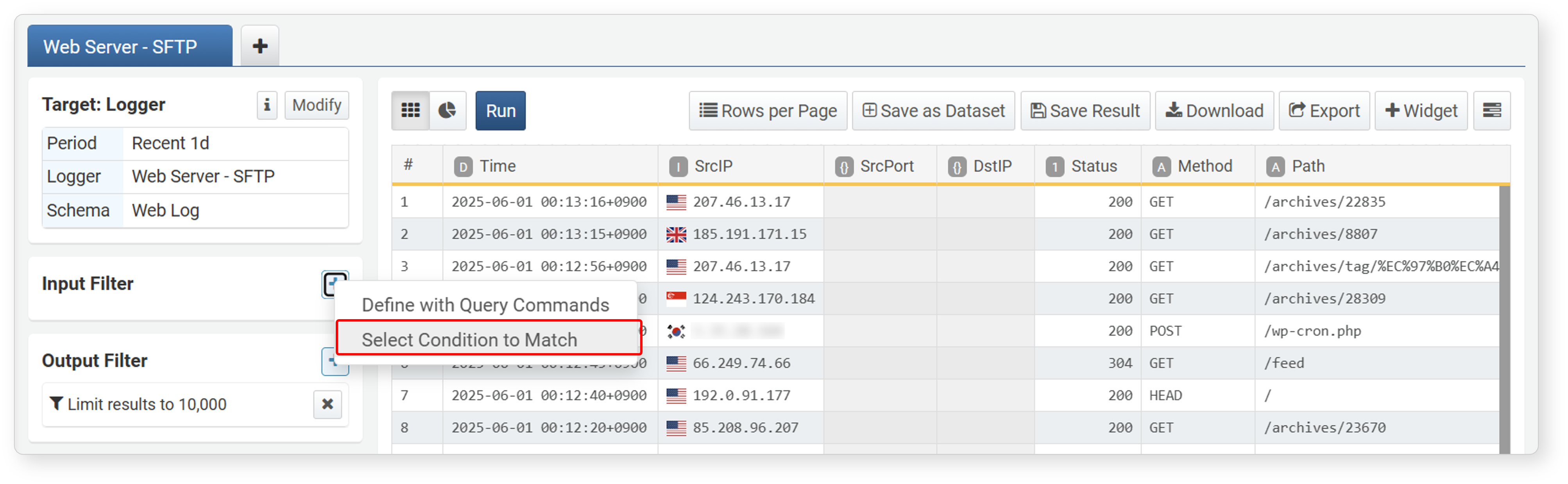
-
Select filter properties in the input filter.
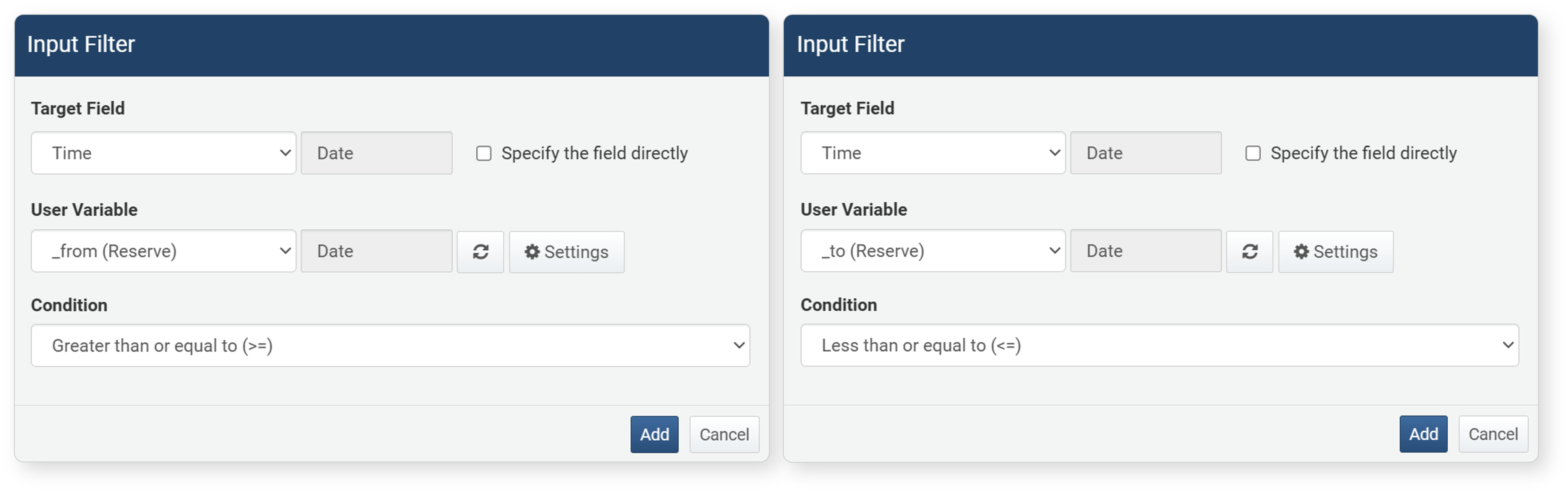
- Target Field: The field to apply the filter to. You can also click Enter Field Directly to enter it manually.
- User-defined Variable: Select a user-defined variable from the list to use for user input via the input control widget.
- Condition: The comparison condition between the target field value and the value entered via the user-defined variable. The left side of the comparison is the target field value, and the right side is the user-defined variable value. Available conditions vary by data type. For details, see Filter Conditions.
- Click the
 button to view or add user-defined variables in a new window.
 - Click the
 button to reload the user-defined variable list.
- Click the
-
Check the results after the filter is applied.
Correlation Filter
A correlation filter allows you to use the analysis results from one pivot screen as a filter in another pivot screen. For example, you can import IPS logs into a pivot screen, aggregate the top 5 attacker IP addresses, and then set those top 5 IPs as a correlation filter in a new pivot tab to search firewall logs containing those IPs.
Correlation filters are similar to correlation analysis in that they perform database operations (join) on two or more pivot data groups (tabs), but are used to narrow the analysis scope by filtering data in the current pivot data group.
To use a correlation filter, you need at least two pivot tab screens. The usage is as follows:
-
In the workspace, select the field to apply the correlation filter to, then click Correlation Filter in the popup menu.
-
Enter the settings in the Correlation Filter dialog and click Apply.
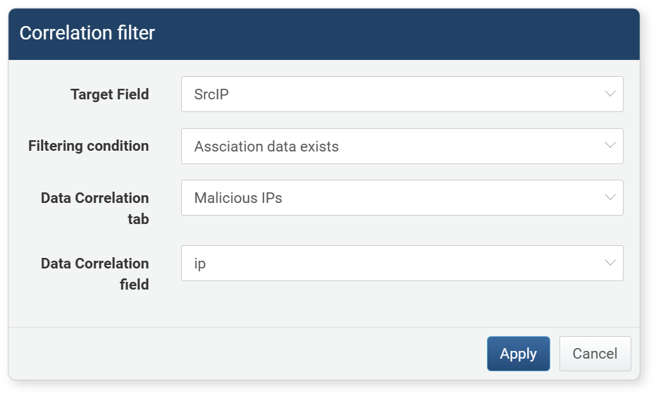
- Target Field: The field to apply the correlation filter to (default: selected field)
- Filter Condition: Search condition (default: when correlation data exists)
- When correlation data exists: Checks if the target field value matches the correlation analysis field value
- When correlation data does not exist: Checks if the target field value does not match the correlation analysis field value
- Correlation Analysis Tab: The data group (tab) containing the correlation analysis field to compare with the target field
- Correlation Analysis Field: The field containing the value to compare with the target field
-
The pivot tab with the correlation filter applied switches to the correlation analysis screen. Unlike correlation analysis, additional filtering is performed by summarizing only the necessary data. You can perform filtering, sorting, and additional correlation analysis as in the original pivot screen.
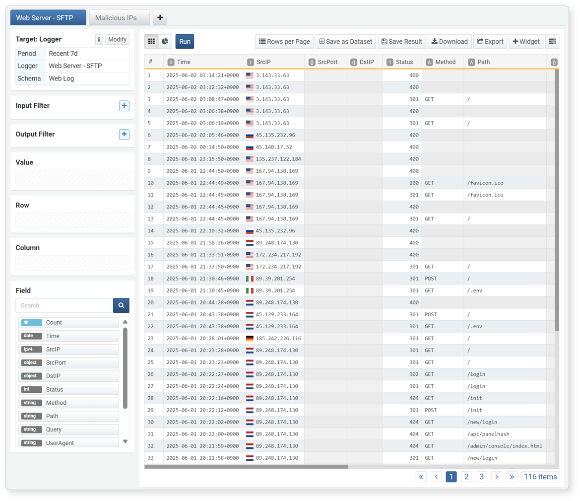
- Click Back in the upper left to return to the screen before applying the correlation filter.
- For available operations, see Correlation Analysis.
Expression
When the data type is date, expressions are provided to truncate imported date data by time unit, calculate time differences, or convert to strings. Expressions help analyze time data more precisely and transform or compare data as needed.
Time Unit Truncation
This expression is useful for dividing data into time intervals (e.g., 5-minute, 1-hour intervals) to generate time series data, mainly used for processing the _time or Time field.
Click Cut date unit in the popup menu of a date-type field or data column to set it in the dialog.
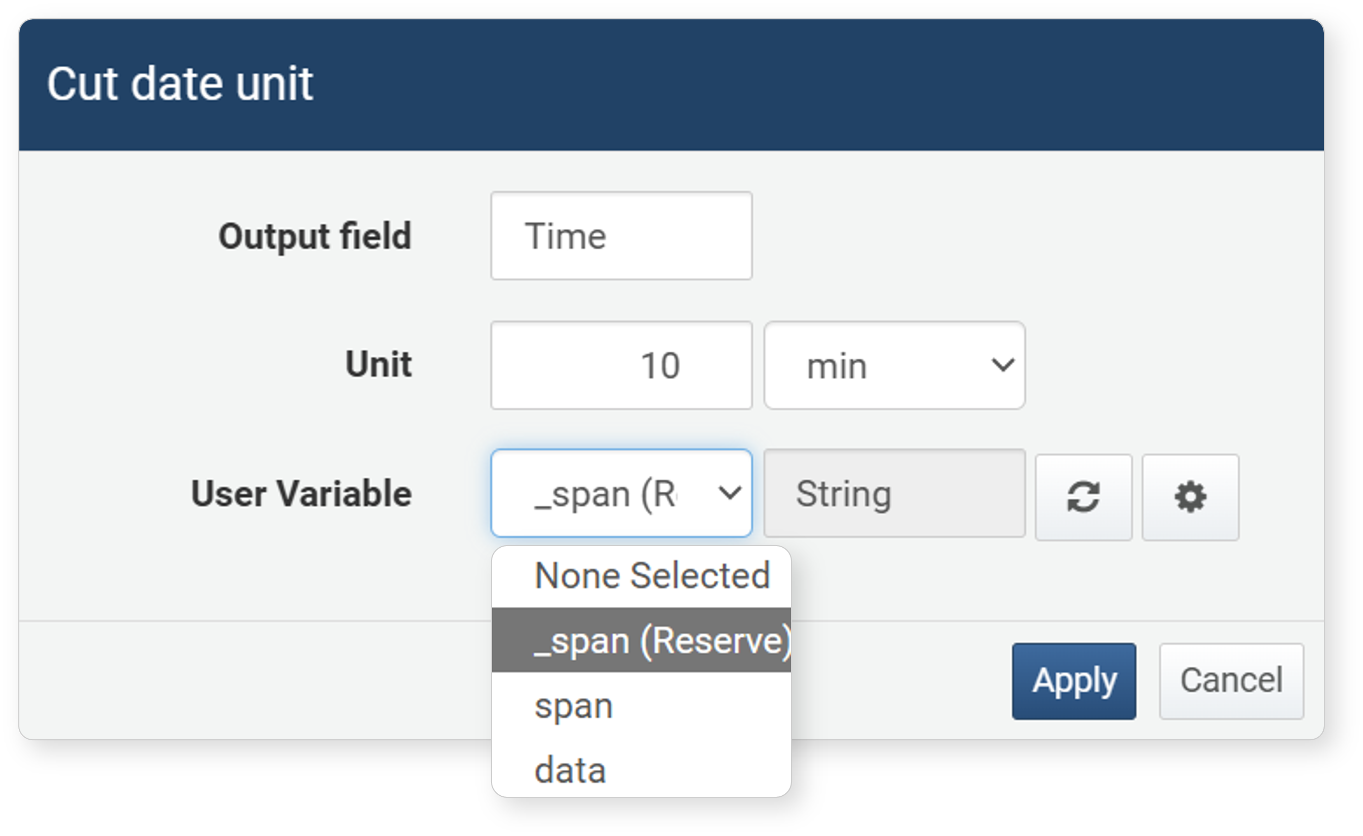
- Output Field (required): The field to apply the expression to
- Unit (required): The base unit of the time interval (default: 10 minutes). Units can be year, month, week, day, hour, minute, second, or millisecond.
- User-defined Variable (optional): To truncate by the time interval entered by the user via the input control widget, select a user-defined variable from the list.
- Click to view or add user-defined variables in a new window.
- Click to reload the user-defined variable list.
- Click
The values entered in the Time Unit Truncation dialog are converted into a query and registered in the input/output filter as follows: eval Time = datetrunc(Time, $("_span_", "10m"))
Since the datetrunc() function takes a string as a parameter, only variables of type string are shown in the user-defined variable list.
Time Difference Calculation
This expression calculates and displays the time difference between the current time and the selected field value in a specified time unit (e.g., seconds, minutes, hours, days). For example, you can calculate the difference between the current time and the recorded time in minutes or display it in hours. This is useful for quickly checking the time difference between specific events.
Click Time Difference Calculation in the popup menu of a date-type field to set it in the dialog.
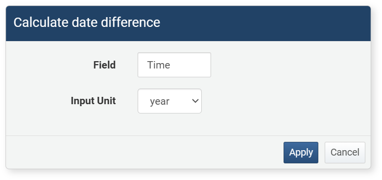
- Field: The field to apply the expression to
- Unit Input: The unit for time difference calculation (default: year). Units can be year, month, week, day, hour, minute, second, or millisecond.
The values entered in the Time Difference Calculation dialog are converted into a query and registered in the input/output filter as follows: eval Time = datetdiff(Time, now(), "min")
String Conversion
This expression converts date values to string format, allowing you to integrate with other data formats or output date data in a specific format. For example, you can convert date data like "2025-01-22 15:30:00" to "January 22, 2025" or change it to another output format. This is useful for displaying time data in a readable way or outputting data in a specific format.
Click String Conversion in the popup menu of a date-type field to set it in the dialog.
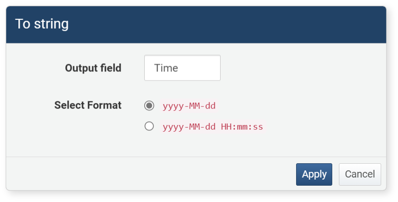
- Output Field: The field to apply the expression to
- Format Selection: The format to convert to (default: yyyy-MM-dd)
The values entered in the String Conversion dialog are converted into a query and registered in the input/output filter as follows: eval Time = string(Time, "yyyy-MM-dd")
Sorting
You can easily sort and manage fields of the retrieved data. This menu allows you to quickly sort the required data or effectively manage the fields displayed on the screen.
Move Field
Data imported by selecting a schema is displayed in the order defined in the log schema, while data imported as raw is displayed in alphabetical order. When configuring widgets, you may need to move only meaningful fields to the front or change the order. Field movement consists of four items.
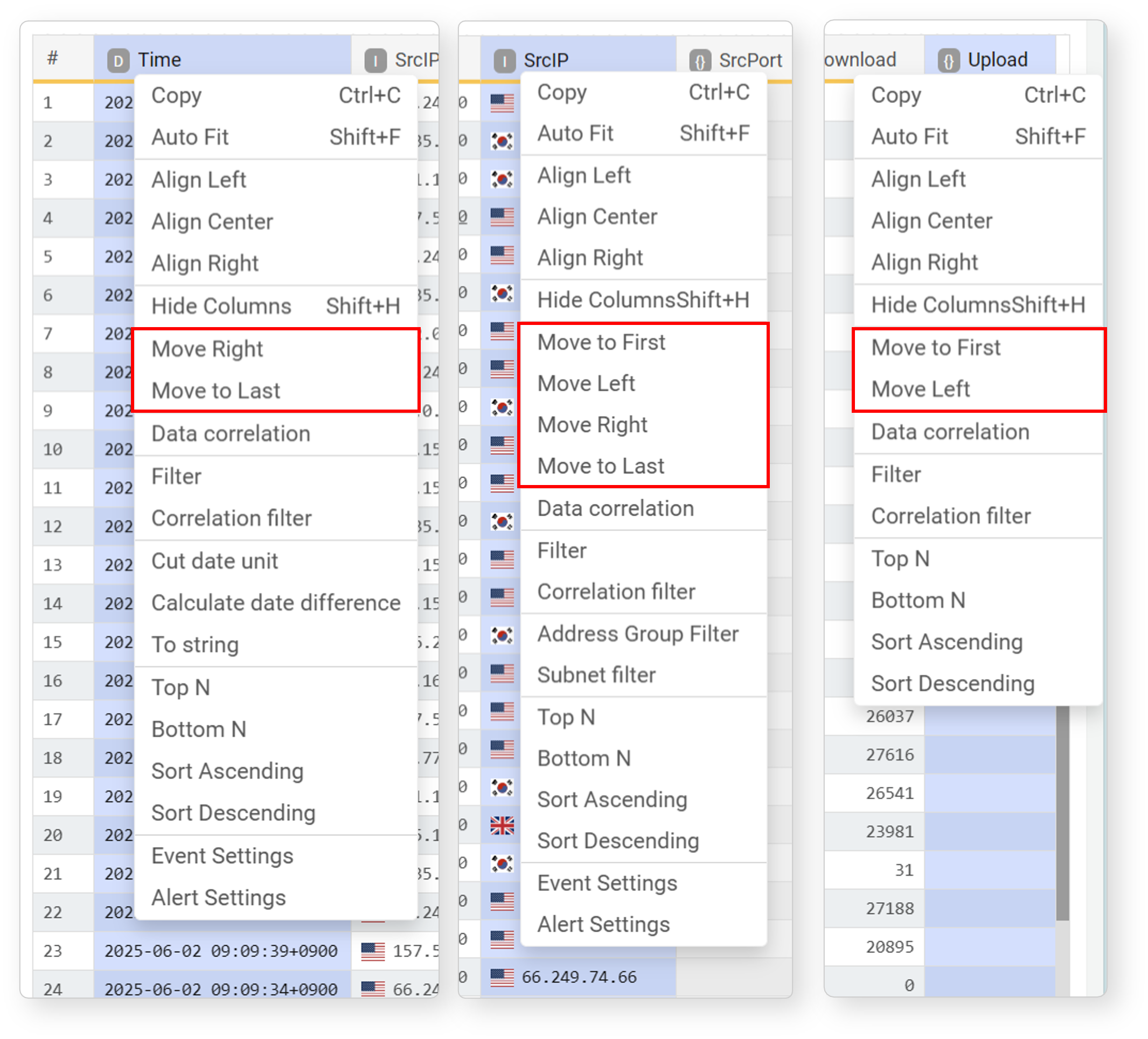
- Move to First: Move the selected field to the far left of the list.
- Move Left: Move the selected field one position to the left.
- Move Right: Move the selected field one position to the right.
- Move to Last: Move the selected field to the far right of the list.
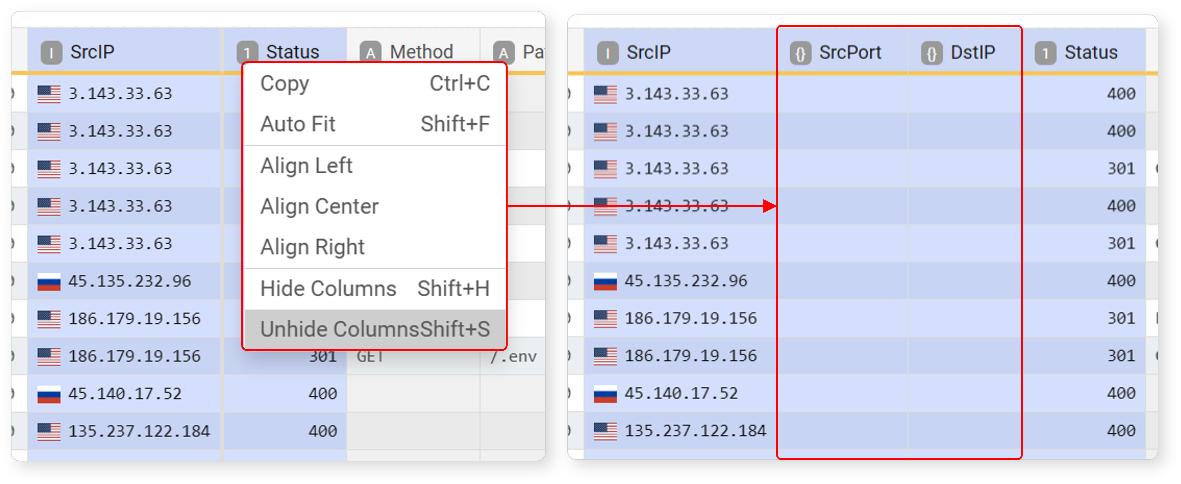
Hide/Show Field
To hide a field, select the field to hide and click Hide in the popup menu or press Shift+H. Hidden fields are indicated by a bold solid line.
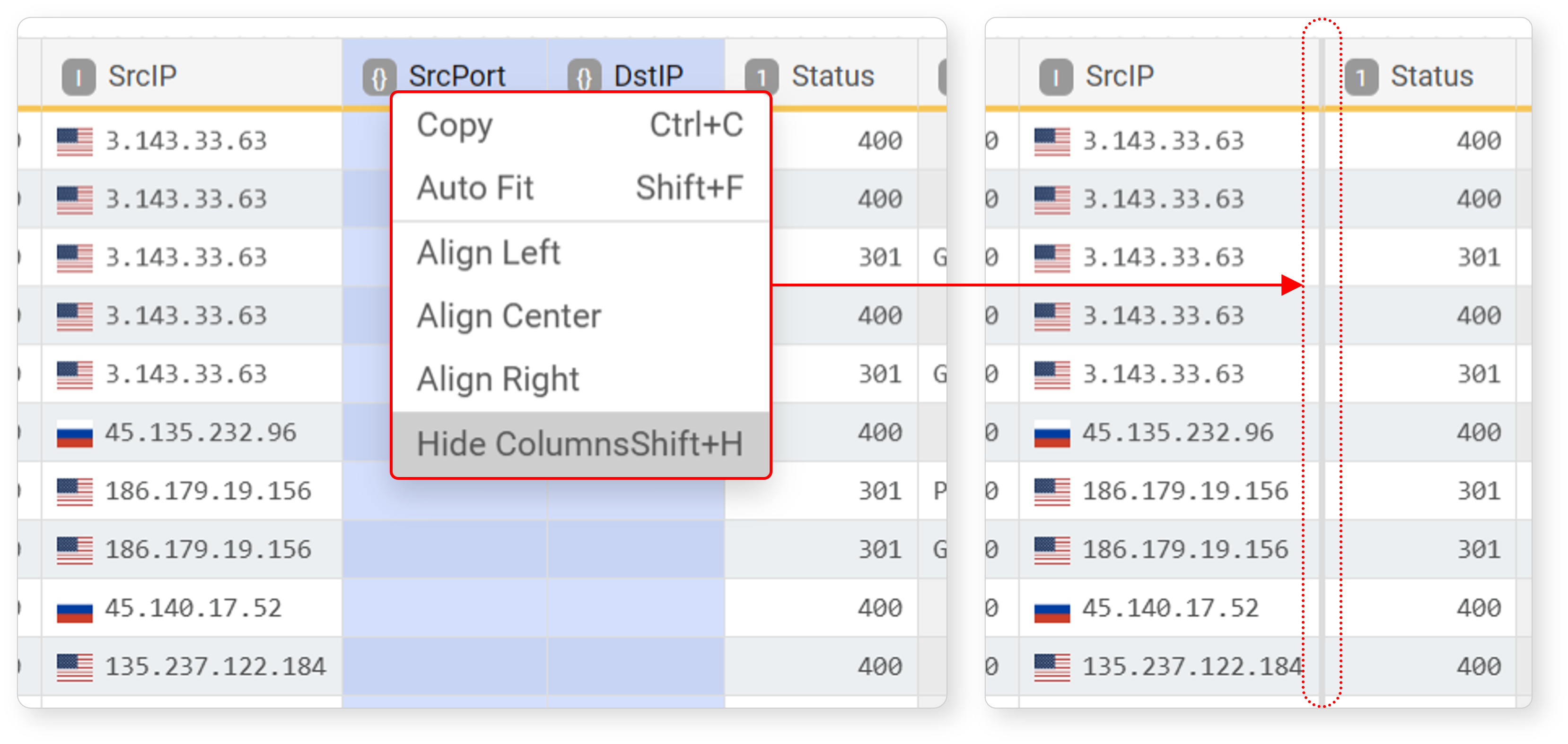
To show a hidden field again, select the fields to the left and right of the hidden field, then click Unhide in the popup menu or press Shift+S.
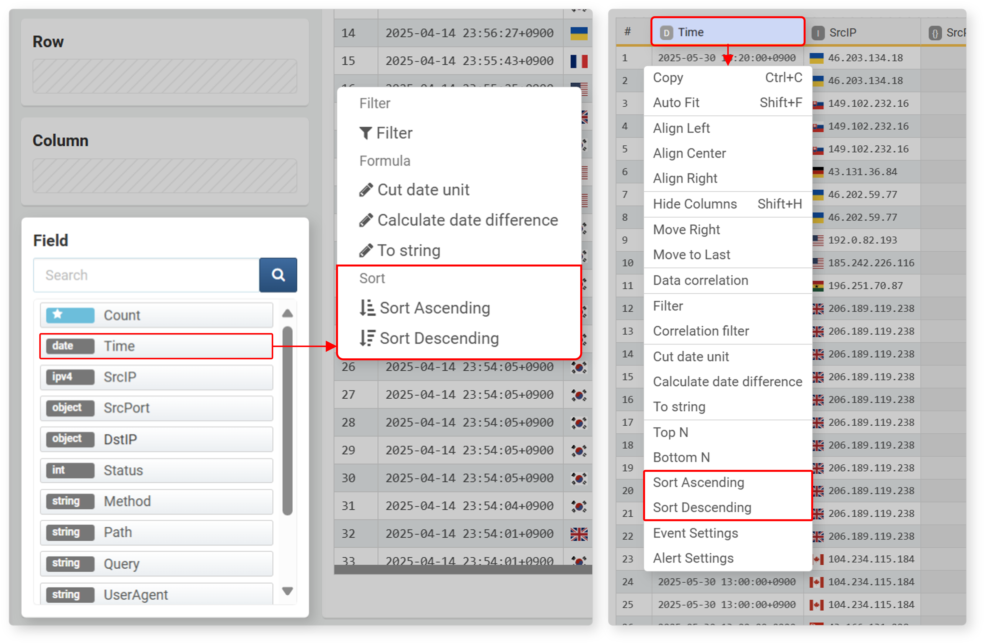
Ascending/Descending
Imported data is displayed in descending order by time (default: descending). To change the sort order based on a specific field, select the field from the field list or workspace, then click Ascending or Descending in the popup menu.
Ascending/descending sort is converted into a sort query and registered in the input/output filter as follows.
| Sort | Query |
|---|---|
| Sort Ascending | sort FIELD_NAME |
| Sort Descending | sort -FIELD_NAME |
Top N/Bottom N
Top N and Bottom N are used to select records with the highest (descending) or lowest (ascending) values for a specific field.
To select top/bottom records:
-
In the workspace, select the field, then click Top N or Bottom N in the popup menu.
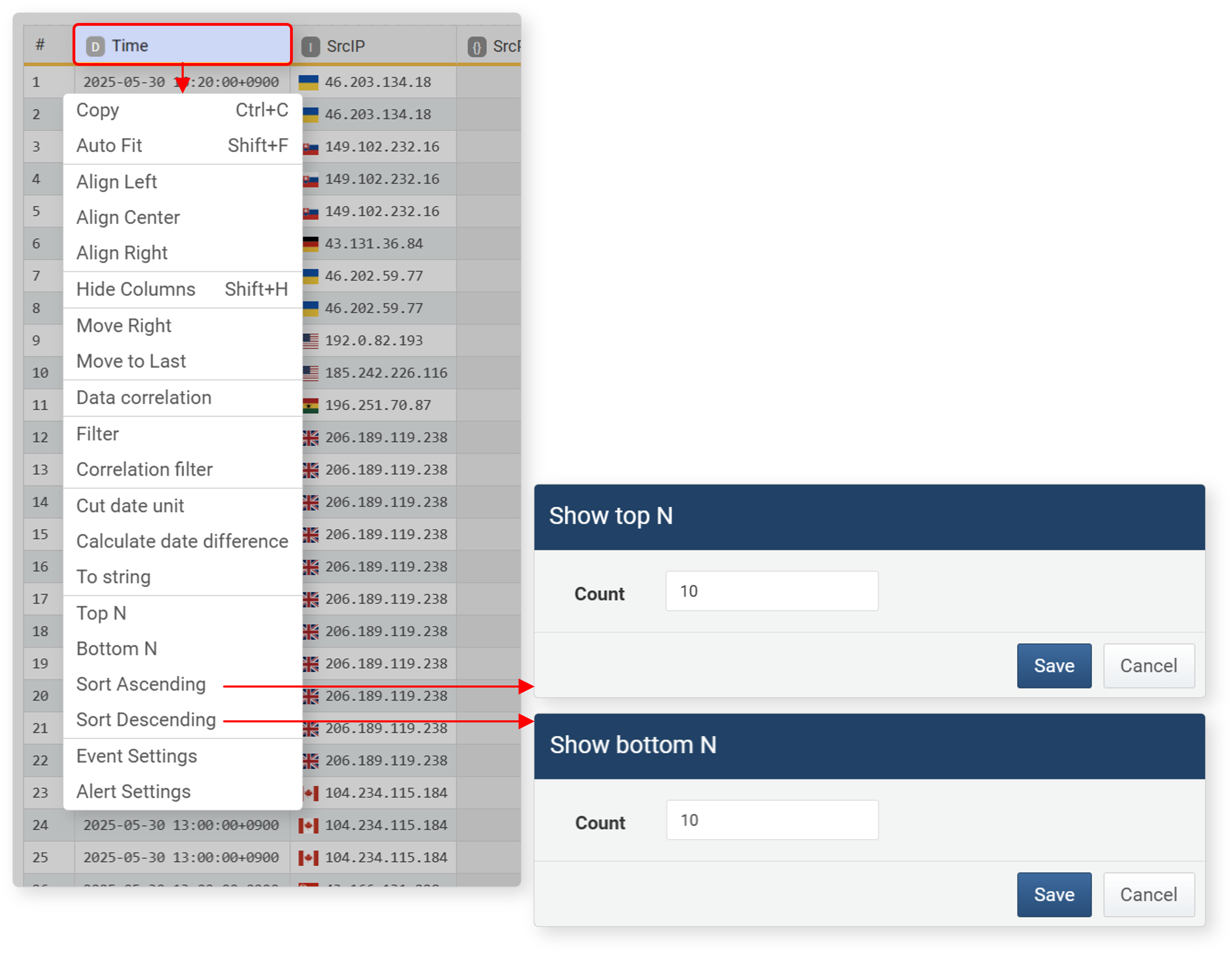
-
In the Show Top N Only or Show Bottom N Only dialog, enter the number to view and click Save.
Top N/Bottom N settings are converted into queries and registered in the input/output filter.
| Sort | Query |
|---|---|
| Top N | sort limit=N -FIELD_NAME |
| Bottom N | sort limit=N FIELD_NAME |
Left/Center/Right Alignment
Most field values are left-aligned, and numbers such as integers and floats are right-aligned. To change the alignment, select the field, then choose Left Align, Center Align, or Right Align in the popup menu.

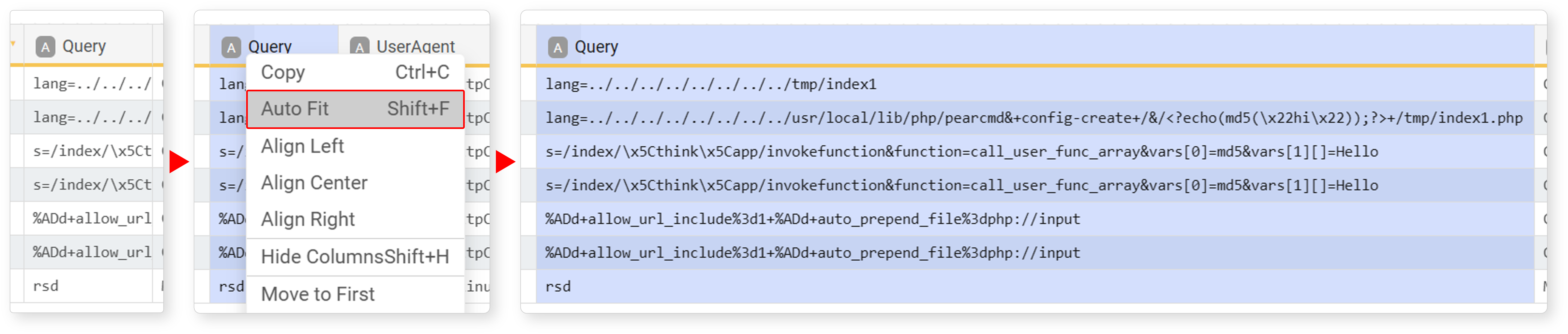
Auto Fit
Fit adjusts the field width to match the length of the field data. Select the field, then click Auto Fit in the popup menu or press Shift+F to adjust the field width to the longest data in the field.
Analysis Tools
In addition to filters, expressions, and sorting, the following features are useful for analysis.
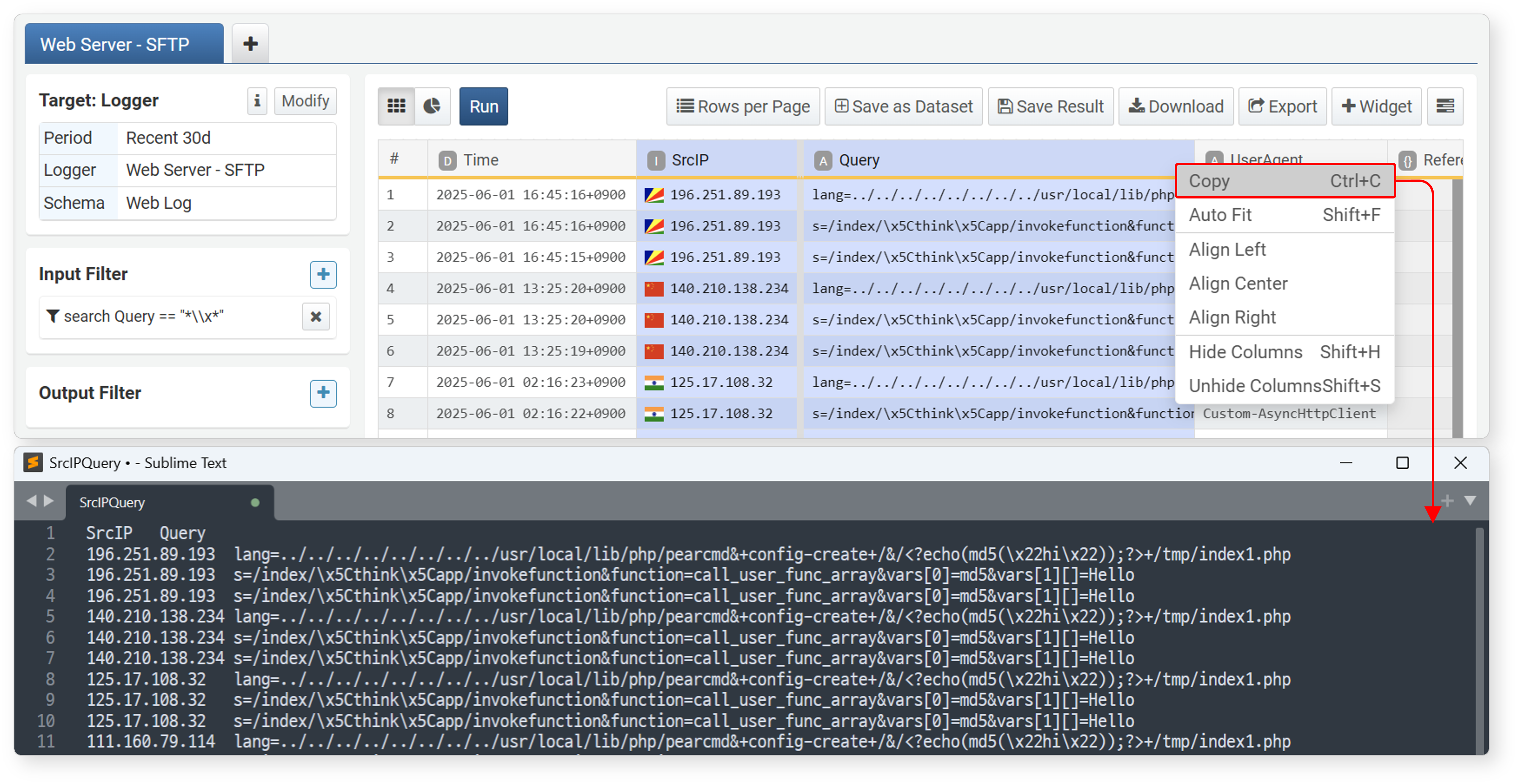
Copy
Select a field, then click Copy in the popup menu or press Ctrl+C to copy the displayed values in the selected field column to the clipboard in TSV (tab-separated text) format.
Copy IP Information
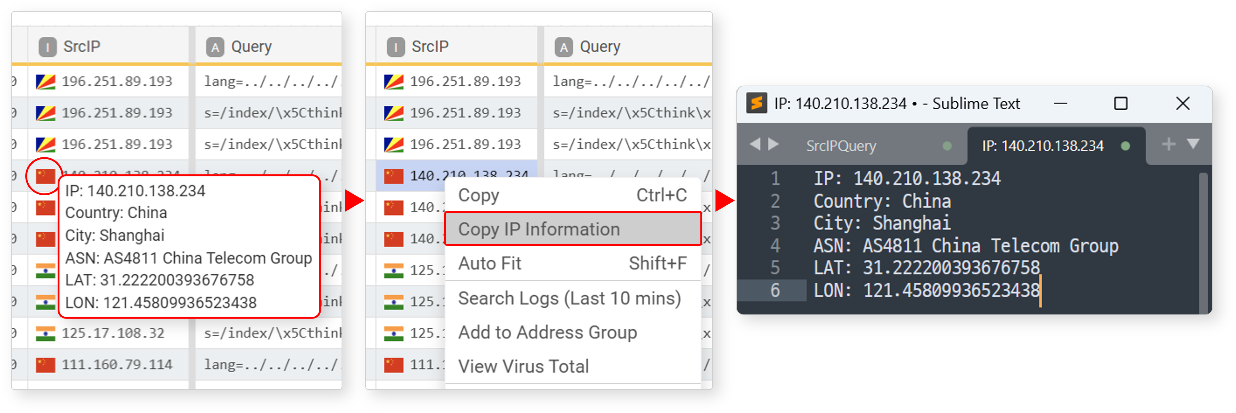
In an IP address type field, hovering over the flag next to the IP address displays its location information (IP address, country, city, ISP, latitude, longitude). Click Copy IP Information in the cell popup menu to copy the IP address location information to the clipboard.
Search Logs (Last 10 mins)
In an IP address type field, select a cell and click Search ±10 Minutes in the popup menu to search and display all data containing the IP address within 10 minutes before and after the record's timestamp. This helps you understand the context around a specific event.
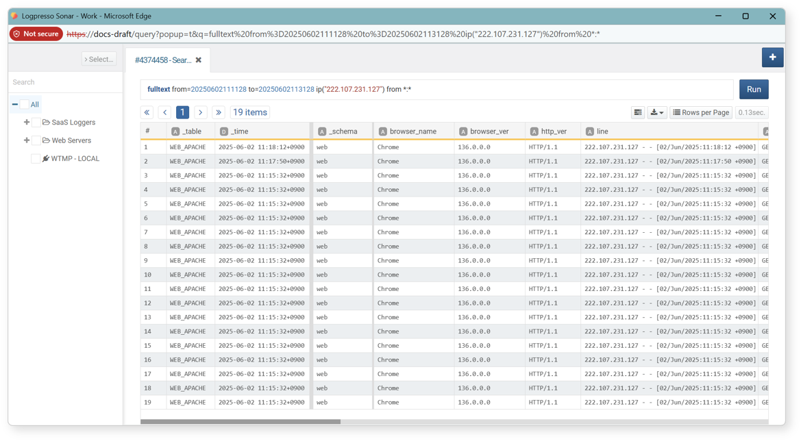
The result is as follows (related command: fulltext).
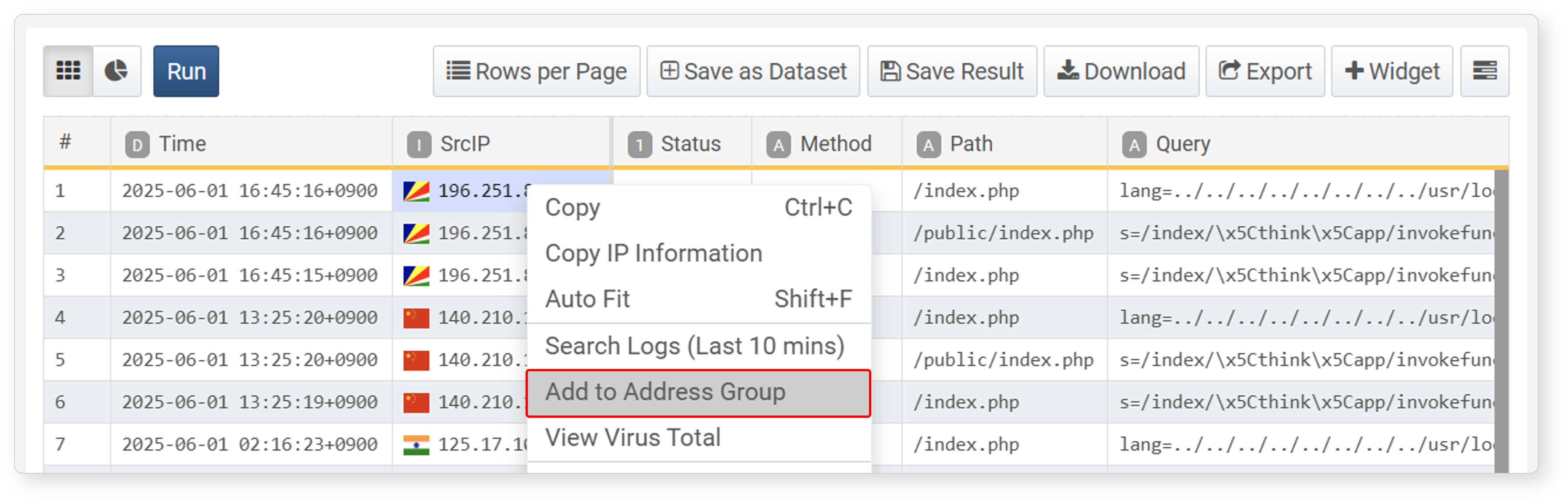
Register Address Group
In an IP address type field, you can register the selected cell's IP address to an address group. This allows you to group IP addresses for easier management and search in the future.
To register an IP address to an address group:
-
In an IP address type field, select a cell and click Register Address Group in the popup menu.
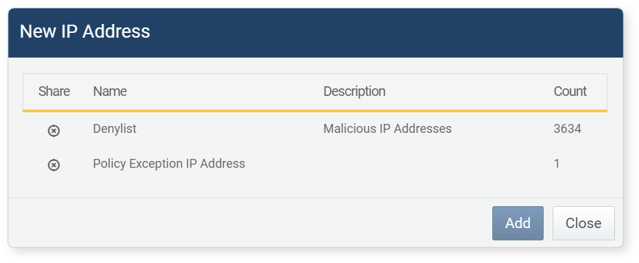
-
In the New IP Address window, select the address group and click Add.
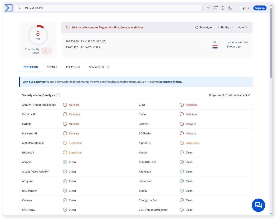
VirusTotal Lookup
In an IP address type field, select a cell and click VirusTotal Lookup in the popup menu to check threat intelligence information related to the IP address in VirusTotal in a new window. This helps security administrators quickly review suspicious IP addresses and take further action.
The result is as follows.
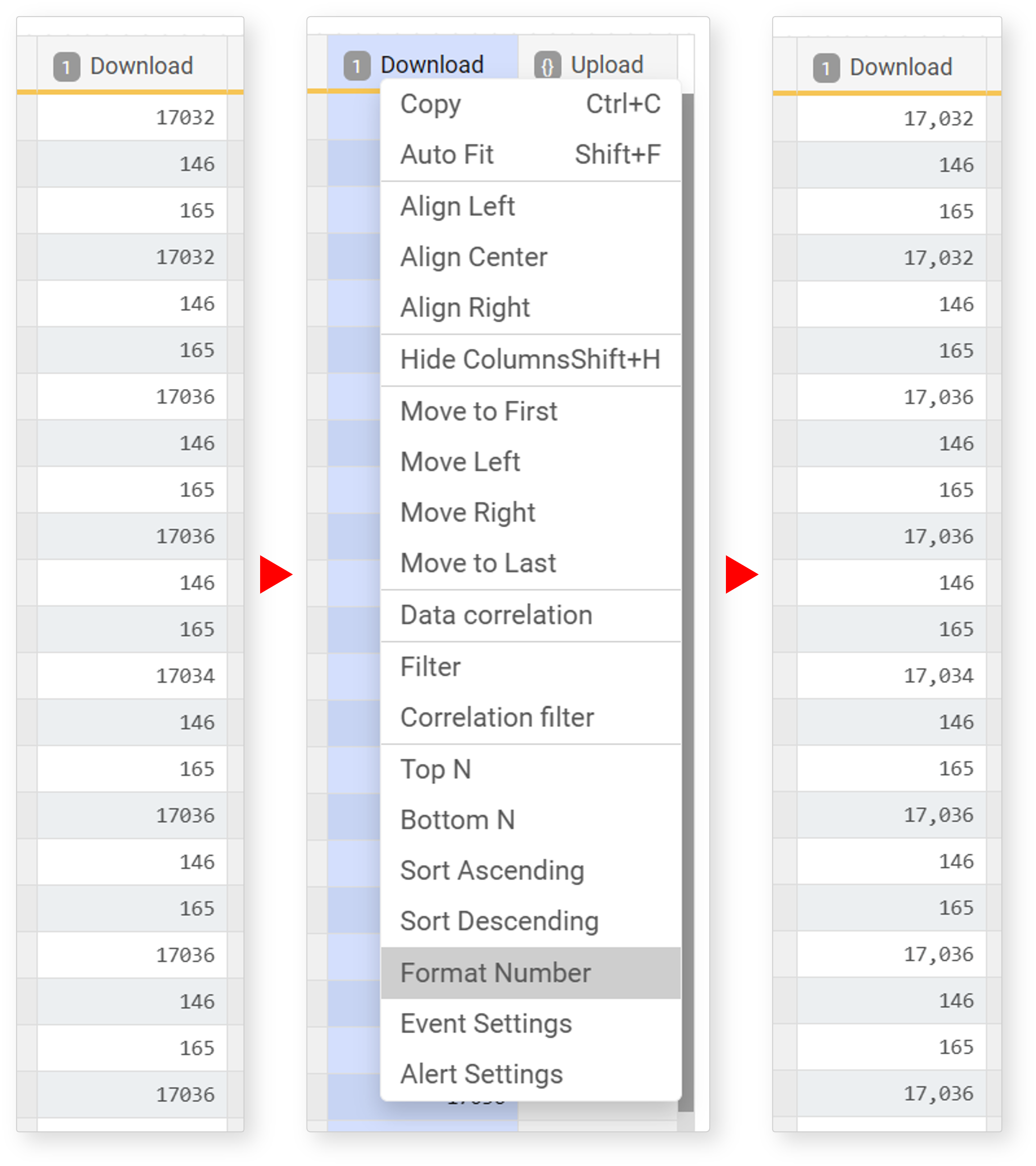
Thousand Separator
Select a number (integer, float) type field, then click Thousand Separator in the popup menu to display numbers with a thousands separator. This is useful for intuitively understanding the size and scale of numbers.
User-defined Variables
User-defined variables are used to control the information displayed by widgets according to values entered by users in the input control widget (e.g., specific date and time, specific IP address).
Dashboard widgets can be configured from the pivot screen (the widget editor also uses the pivot screen as the default). User-defined variables can be specified when setting dynamic filters or time unit truncation.
View/Search Variable List
To view user-defined variables:
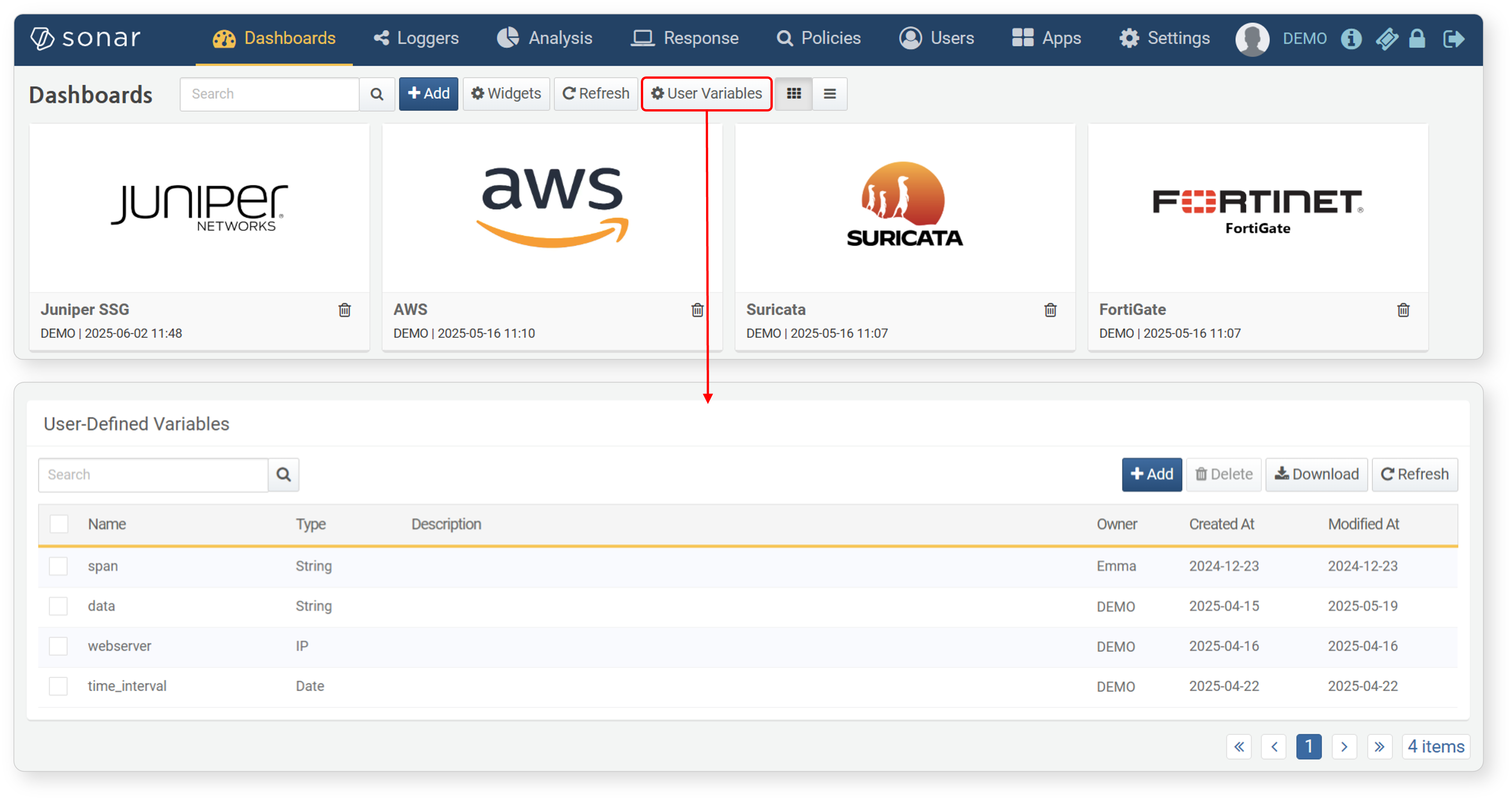
- From the dashboard screen
-
Click User-defined Variables in the dashboard to view the list in a new window.
- From the pivot screen
-
When setting a dynamic filter or time unit truncation expression, click the
button to view the list in a new window.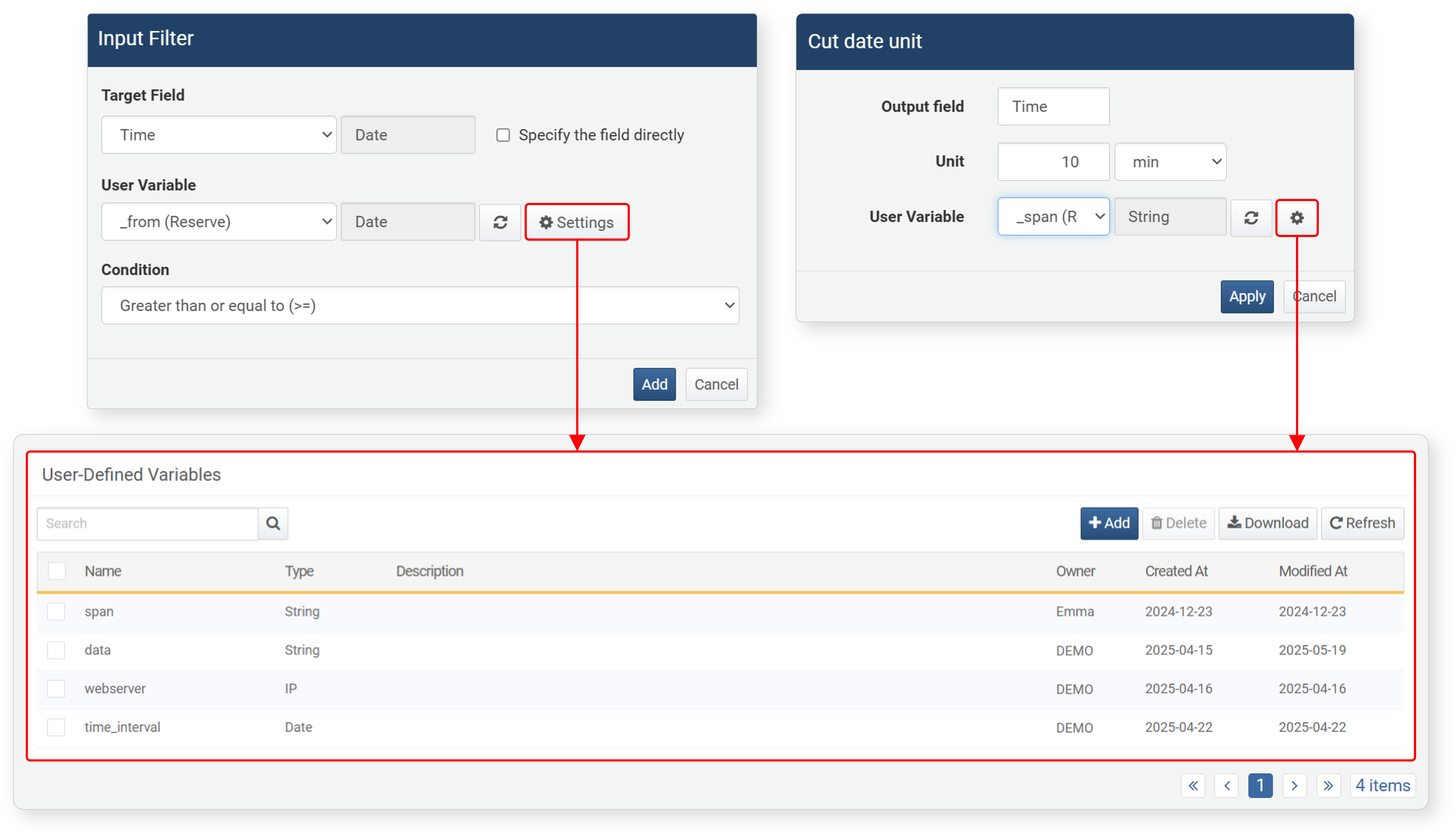
To find a specific user-defined variable in the list, use the search tool in the toolbar. The search tool finds and displays variables whose name contains the search term. The search tool is case-sensitive.
Add Variable
To add a user-defined variable:
-
In the View Variable List screen, click Add.
-
In the Add User-defined Variable screen, enter/select the properties of the variable and click OK.
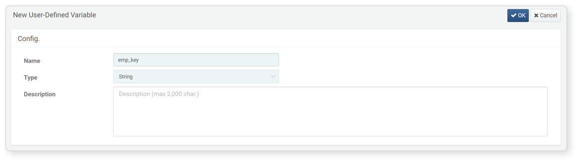
- Name: Unique name of the user-defined variable (up to 50 characters)
- Type: Type of the user-defined variable (default: string). Specifies the type of value to be entered by the user.
- Description: Detailed description of the user-defined variable (up to 2,000 characters)
Edit Variable
To edit a user-defined variable:
- In the View Variable List screen, click the name of the variable to edit.
- In the Edit User-defined Variable screen, modify the information and click OK. The name cannot be changed.
Delete Variable
To delete a user-defined variable:
- In the View Variable List screen, select the checkbox for the variable to delete.
- Click Delete in the toolbar.
- In the Delete User-defined Variable dialog, check the list of variables to delete and click Delete. Click Cancel to abort.
Data Analysis
This section explains how to define a pivot table after data processing to summarize relationships between items, aggregate data, or perform correlation analysis with other data to transform it into meaningful forms.
Data analysis and data processing are only distinguished for convenience; in practice, they are performed simultaneously.
Pivot Table
The pivot table feature allows you to visually reorganize data by dragging and dropping fields, making it easy to analyze data. It works similarly to the pivot table in MS Excel and is very useful for quickly analyzing large amounts of data and extracting important patterns or statistics. The following explains how to configure a pivot table and check aggregation results.
Matrix
To configure a pivot table, first set up the matrix needed for analysis. Typically, fields used as key values or classification criteria are specified as dimensions. Select the fields to analyze from the field list at the bottom left and drag them to Rows and Columns to automatically generate a pivot table.
-
Rows: Analysis criteria fields. Records are created based on combinations of row field values.
-
Columns: Analysis target value fields. Columns are created with the field names of each column field. Duplicate values are considered as one and converted into a single column. The number of unique values in the analysis target field must be 1,000 or less. If there are more than 1,000 unique values, a pivot table cannot be configured.
-
Clicking a field added to Rows/Columns brings up a popup menu where you can sort field values or remove the field from the matrix settings.
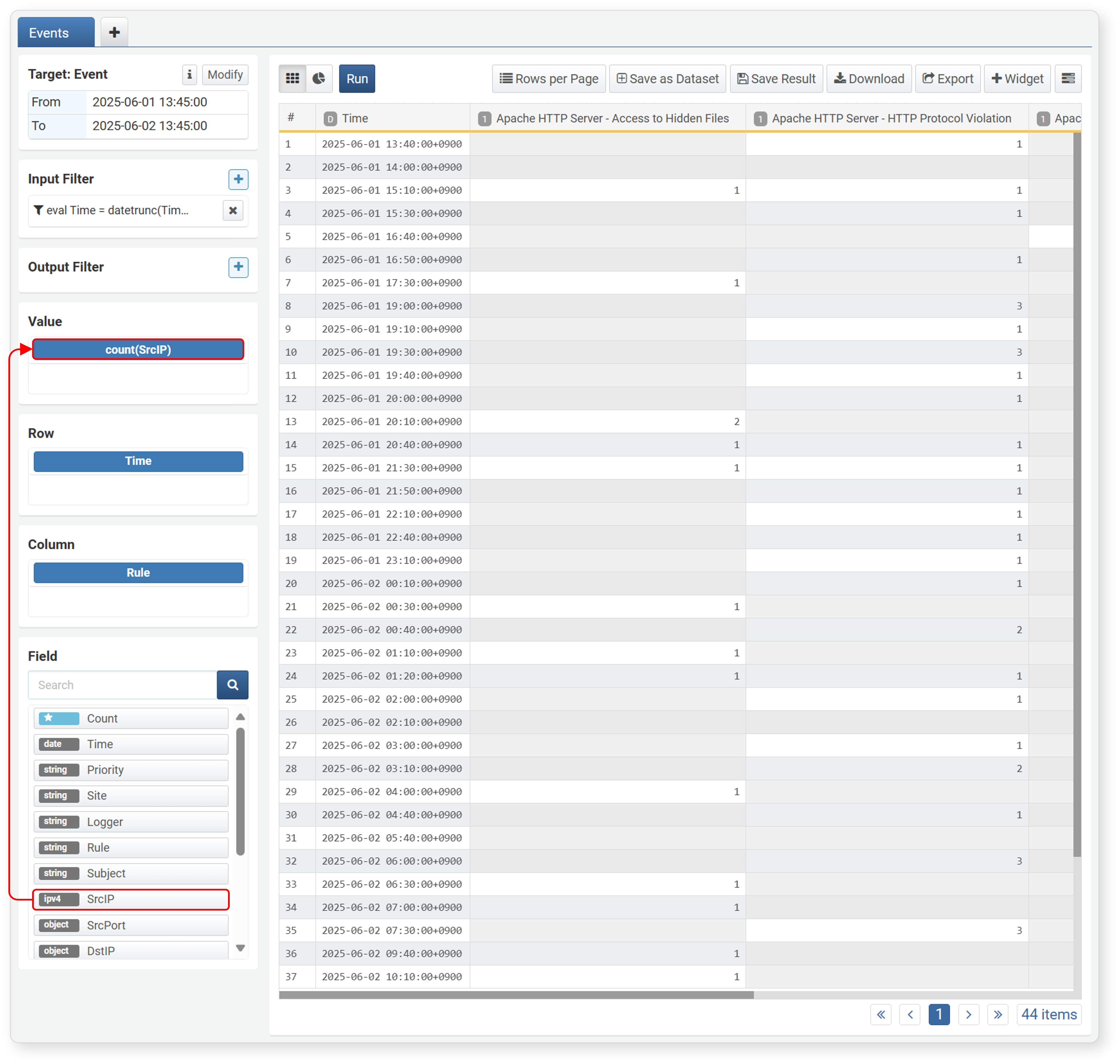
Aggregation Value/Function
After setting up the matrix, select the field to aggregate values. The selected field should generally be of a type that supports aggregate functions. Select a field from the field list and drag it to Values to automatically apply the count() function. If you want to count the number of records containing the column field based on the row field, drag the Count field from the field list to Values.
-
Values: The field to aggregate information according to the matrix
-
Count: Drag the Count field at the top of the field list to Values to display the count for each field in the right panel.
-
Clicking a field added to Values brings up a popup menu to modify the aggregate function for that field. The list of available aggregate functions and their descriptions are displayed. Select the desired function and click Modify to apply it to the pivot table.
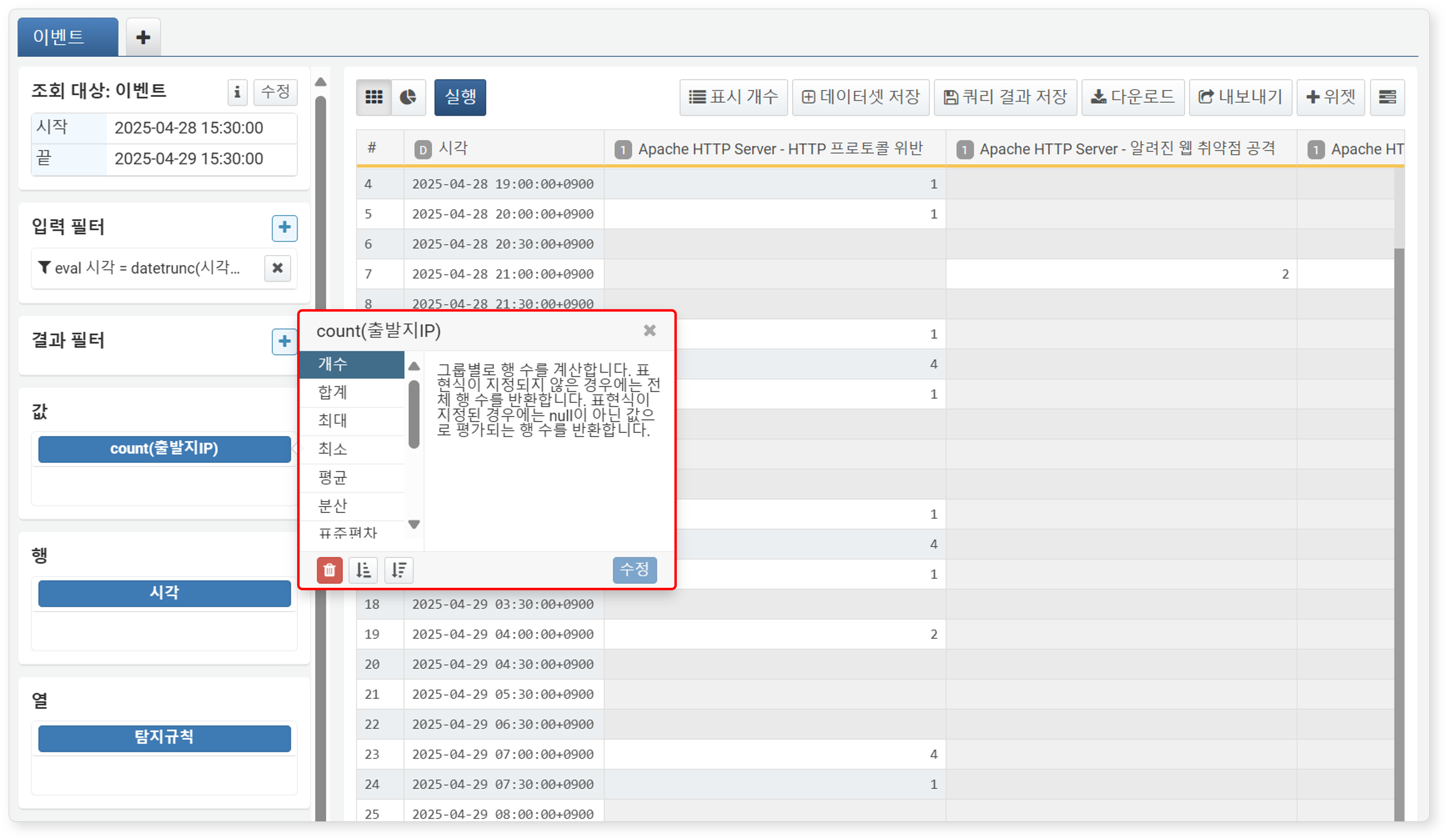
- Click the Trash icon to remove the field from Values.
- Click the Ascending/Descending Sort icon to register a sort statement in the result filter and sort the aggregate values in ascending/descending order.
Supported aggregate functions are as follows:
- Count: Calculates the number of rows per group. If no expression is specified, returns the total number of rows; if an expression is specified, returns the number of rows where the expression evaluates to non-null (count()).
- Sum: Calculates the sum of all expressions in the group. Expressions that are
nullor not numbers (short,int,long,float,double) are ignored (sum()). - Max: Calculates the maximum value among expressions in the group. Null expressions are ignored. May not work as intended when comparing different types (max()).
- Min: Calculates the minimum value among expressions in the group. Null expressions are ignored. May not work as intended when comparing different types (min()).
- Average: Calculates the average of all expressions in the group. Expressions that are
nullor not numbers are ignored (avg()). - Variance: Calculates the variance of all expressions in the group. Expressions that are
nullor not numbers are ignored (var()). - Standard Deviation: Calculates the standard deviation of all expressions in the group. Expressions that are
nullor not numbers are ignored (stddev()). - First Value: Returns the value of the first expression in the group (first()).
- Last Value: Returns the value of the last expression in the group (last()).
- Unique Values: Extracts the set of all unique values in the group. Collects up to 100 items per group and creates an array of unique values. Useful for checking unique values (values()).
- Unique Count: Returns the number of unique values in the group. Useful for knowing the number of non-duplicate values in a field (dc()).
- Estimated Unique Count: Returns the estimated number of unique values in the group. Allows you to estimate the unique count while reducing memory usage (estdc()).
Correlation Analysis
You can integrate data collected from various security devices and perform correlation analysis of security events by applying database operations such as join or union between refined data tables. This helps you identify important patterns or anomalies during the process of combining and filtering data, enabling effective detection of potential threats and quick understanding of complex data.
Correlation Types
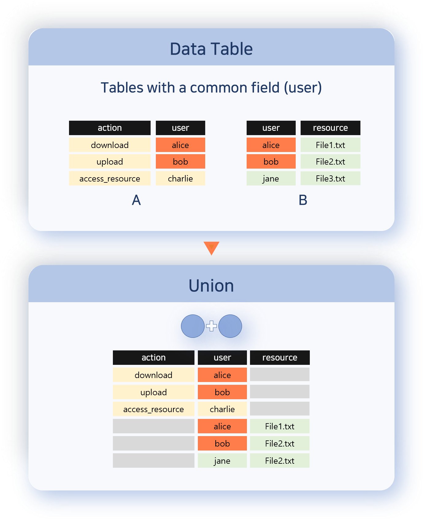
There are six types of correlation: Union, Inner, Left, Right, Full Outer, and Left Only.
- Union
- Union outputs all records from both data sets (data tables in each tab). Each record is retained without modification, and both current data records and correlation analysis data records are included. However, the order of records is not guaranteed.
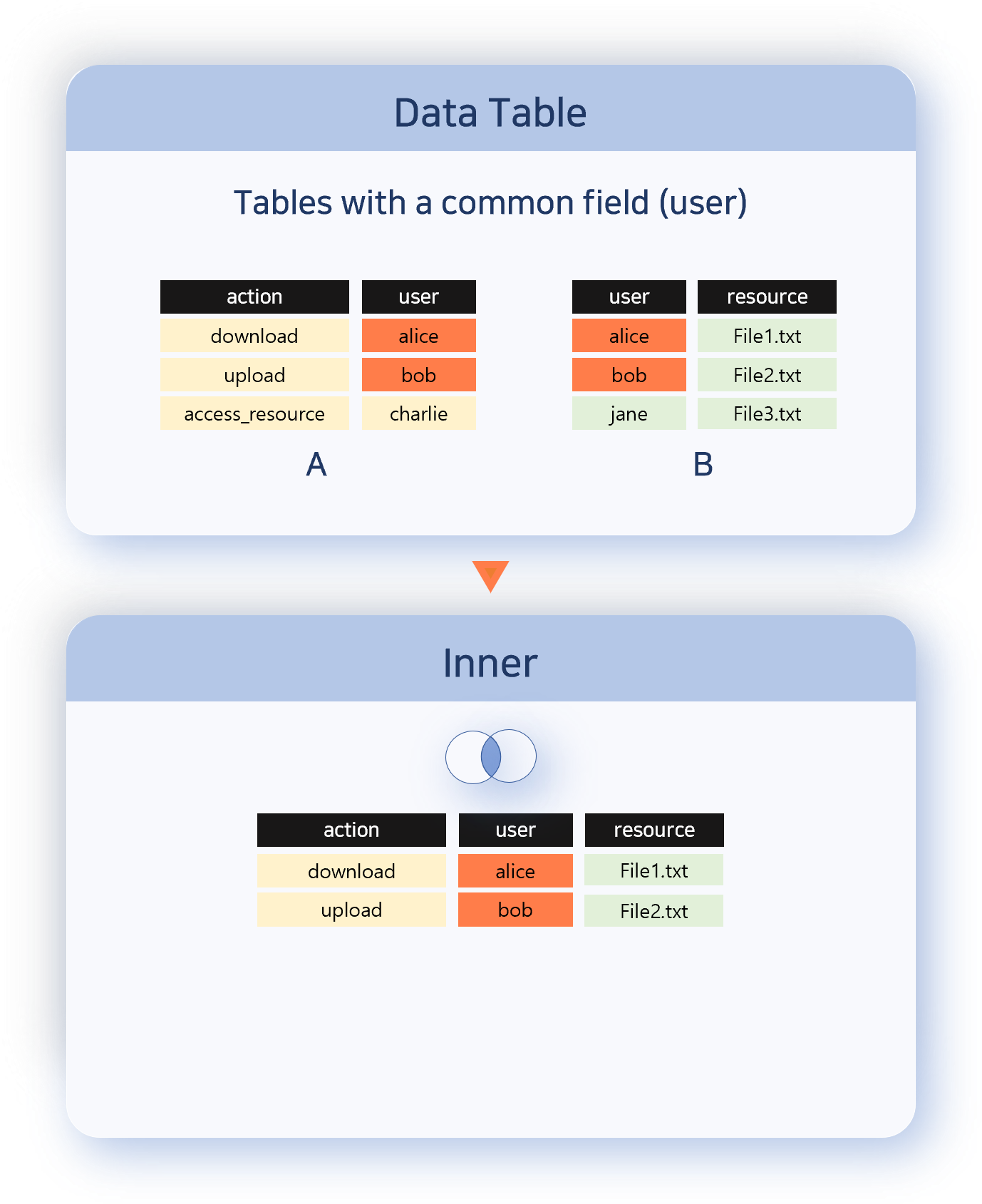
- Inner
- Inner outputs only records where the correlation field values match in both data sets. This allows you to selectively extract only common data.
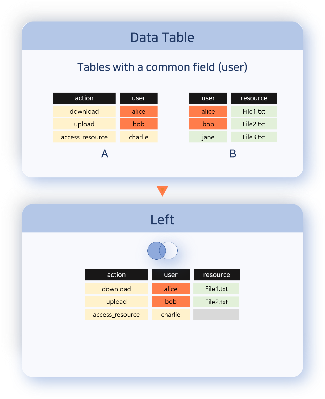
- Left
- Left outputs all records from the left data set. If there is data in the right data set with a matching correlation field value, it is combined with the left data set record.
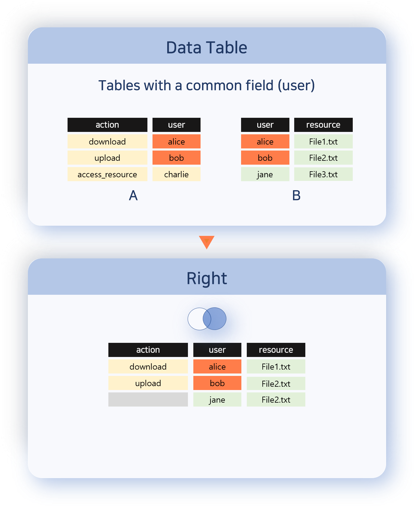
- Right
- Right outputs all records from the right data set. If there is data in the left data set with a matching correlation field value, it is combined with the right data set record.
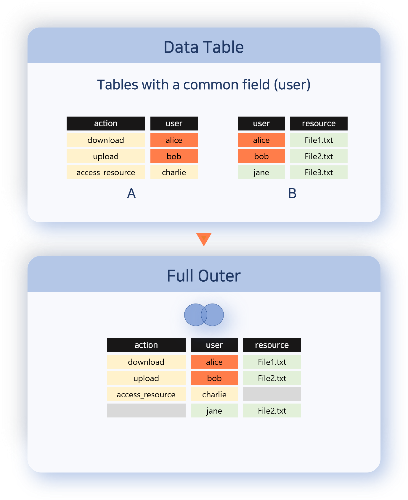
- Full Outer
- Full Outer outputs all records from both data sets (data tables in each tab).
- Data without a correlation field: output as is
- Data with matching correlation fields: combine and output both sides
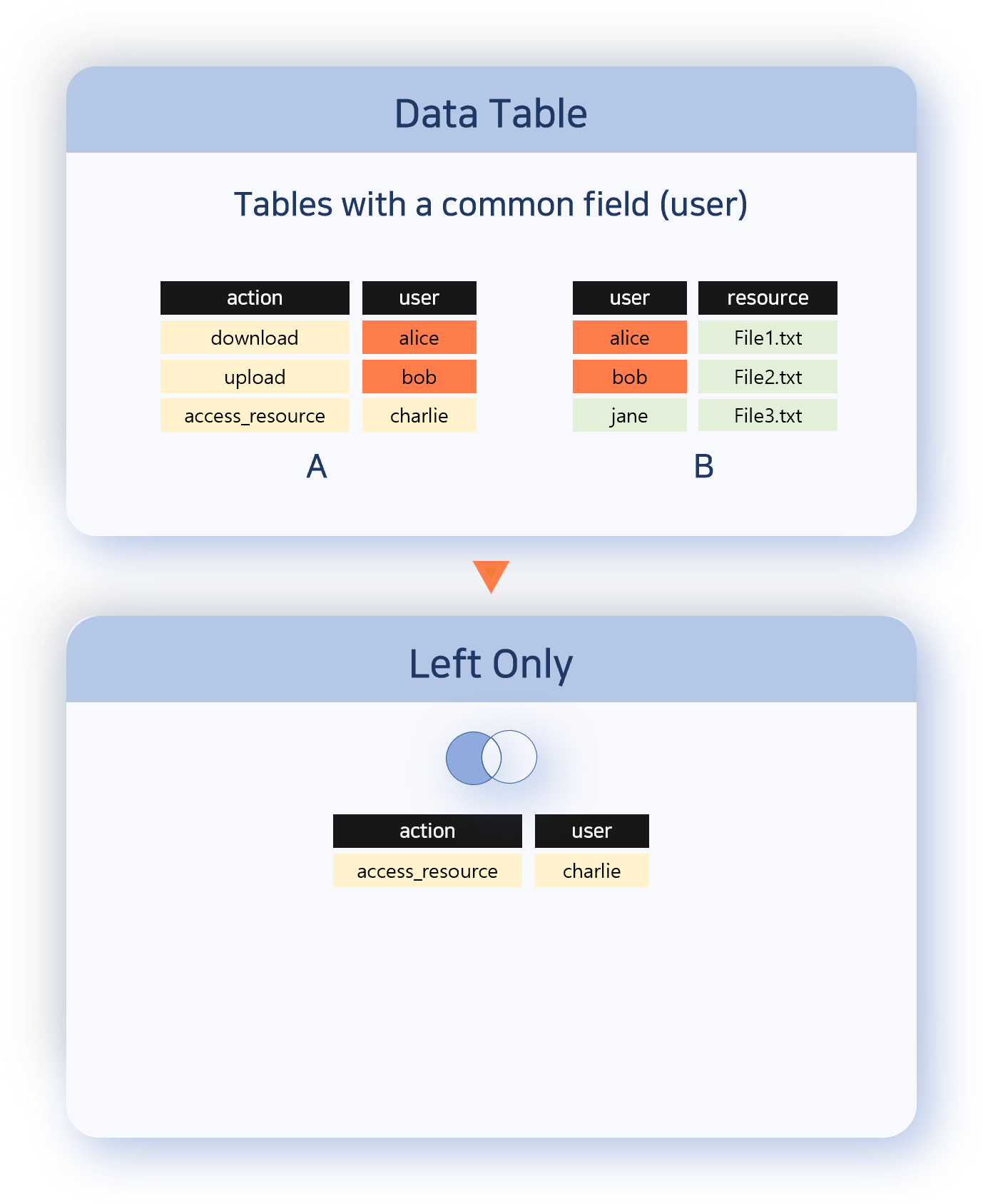
- Left Only
- Left Only is the opposite of Inner and outputs only records from the left data set where there is no matching correlation field value in the right data set.
Performing Analysis
Here, we explain how to check the status of attacks on a web server by correlating an attacker IP address group with web server logs.
- Preparing Data
-
To perform correlation analysis, you need at least two data groups. Open at least two pivot tabs, load the data to be analyzed in each tab, and process it as needed. It is also helpful to rename the pivot tabs for easier identification.
-
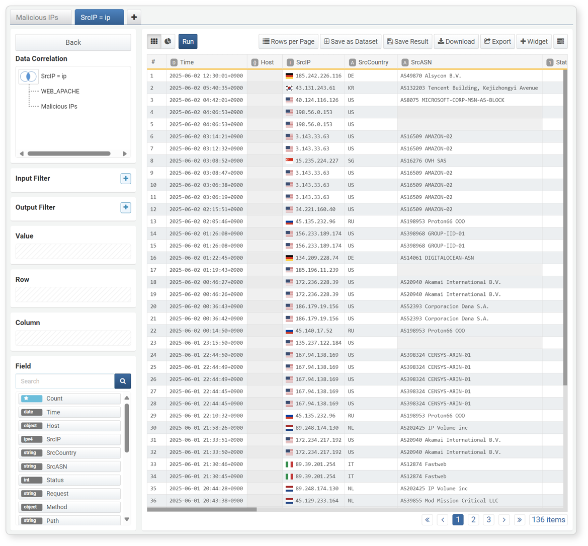
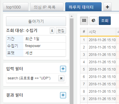
The following shows screens where attacker IP address information and web server logs are retrieved in separate tabs. The attacker IP address data is in the Attacker IP Address List tab, and the web server logs are in the WEB_APACHE tab.
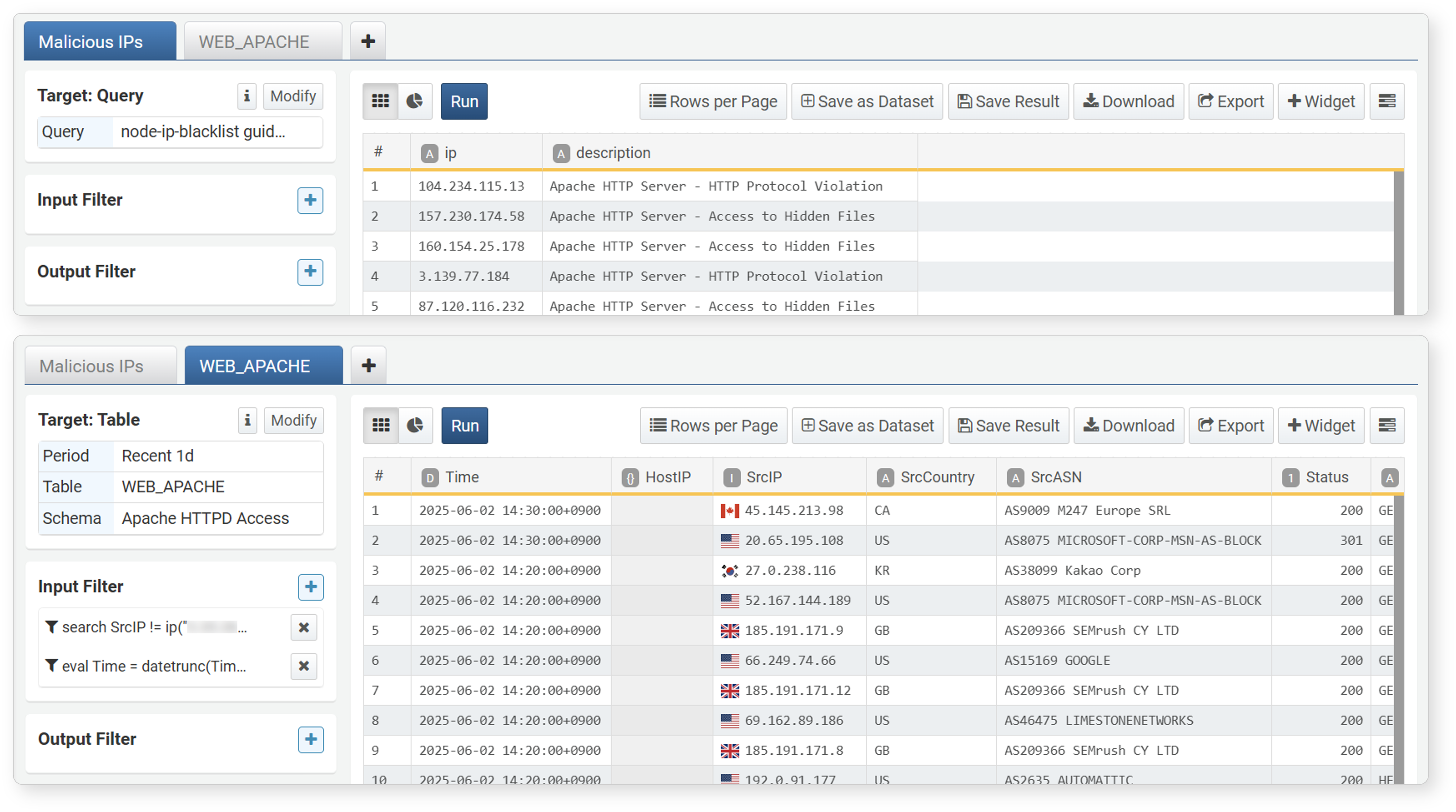 NoteFor the web server logs, an input filter with a time unit truncation expression was applied to check the status in 10-minute intervals.
- Correlation Condition
-
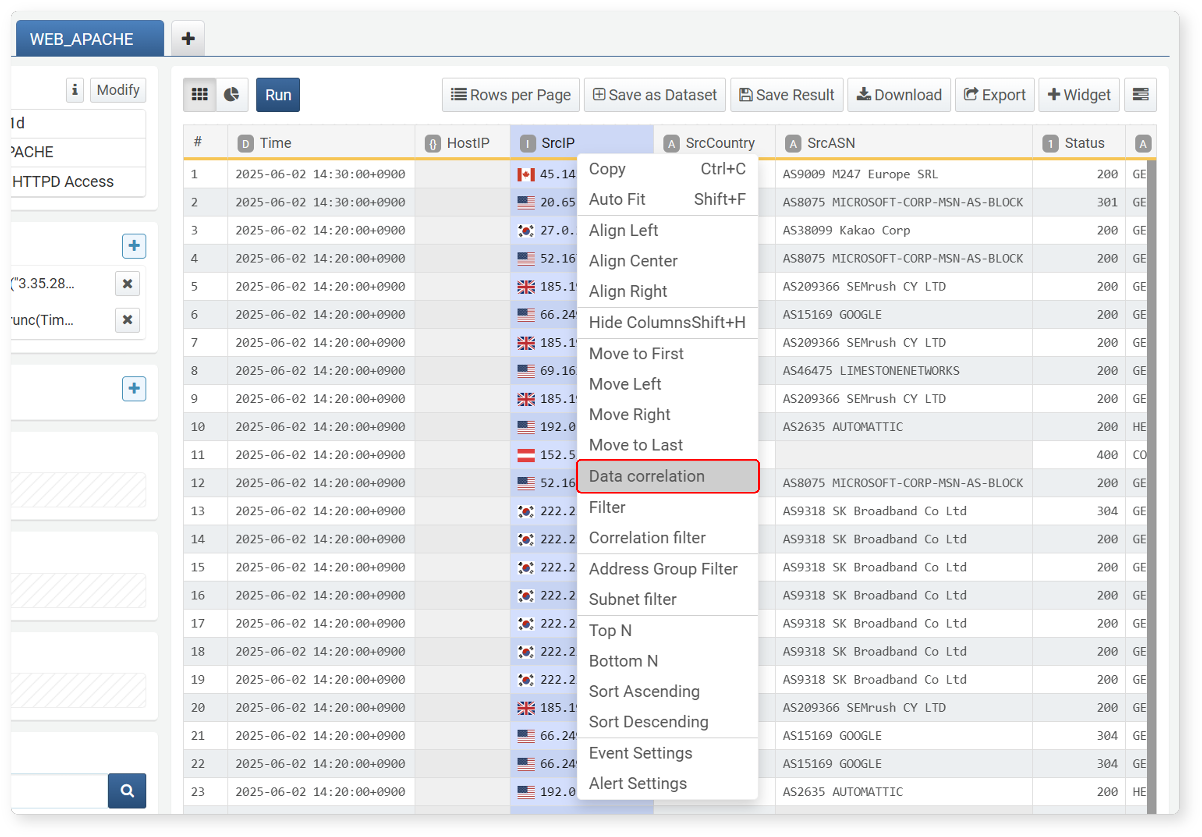
In the data group to be used as the basis for correlation analysis, select the field to be used as the correlation target (in this example, SourceIP in the WEB_APACHE tab), and specify the correlation condition.
-
Click Correlation Analysis in the field popup menu.
-
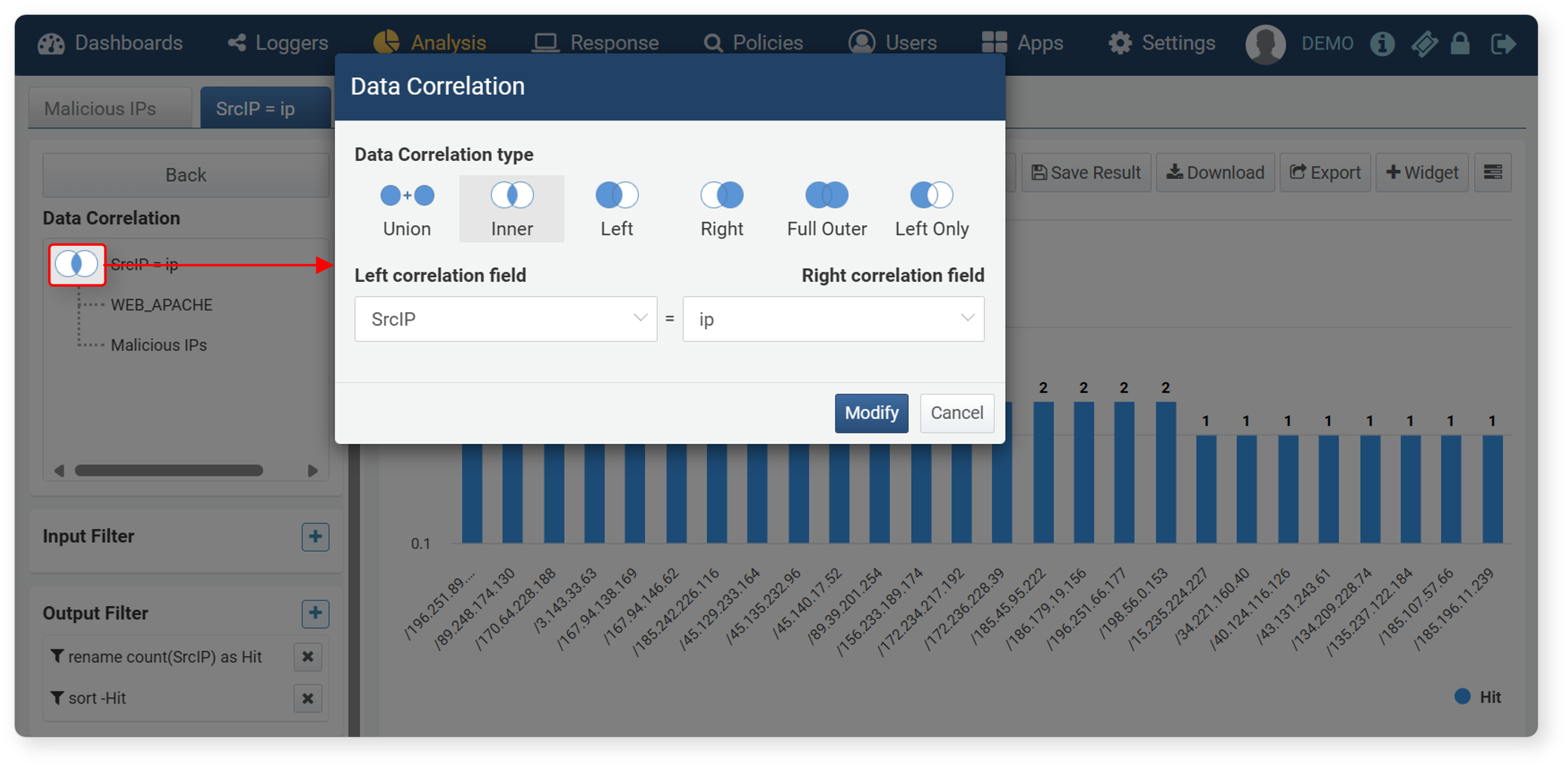
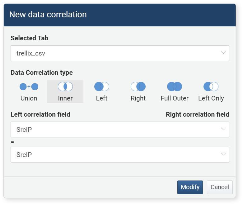
In the Add Correlation Analysis dialog, specify the correlation condition and click OK. In this example, an Inner join is set to match the source IP address in the web server logs with the attacker IP address.
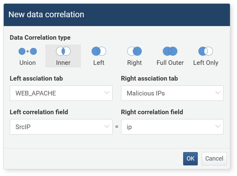
- Correlation Analysis Type: Select one from Union, Inner, Left, Right, Full Outer, Left Only. In this example, Inner is selected.
- Left Correlation Tab: Select the pivot tab to use as the left data group in the correlation analysis
- Right Correlation Tab: Select the pivot tab to use as the right data group in the correlation analysis
- Left Correlation Field: (Except for Union) The field in the left data group to use as the basis for correlation analysis (to be compared with the right correlation field)
- Right Correlation Field: (Except for Union) The field in the right data group to use as the basis for correlation analysis (to be compared with the left correlation field)
- Pivot Table
-
After specifying the correlation condition, click OK to view the correlation analysis results.
-
Now you can analyze the correlation analysis results in the same way as a pivot table.
-
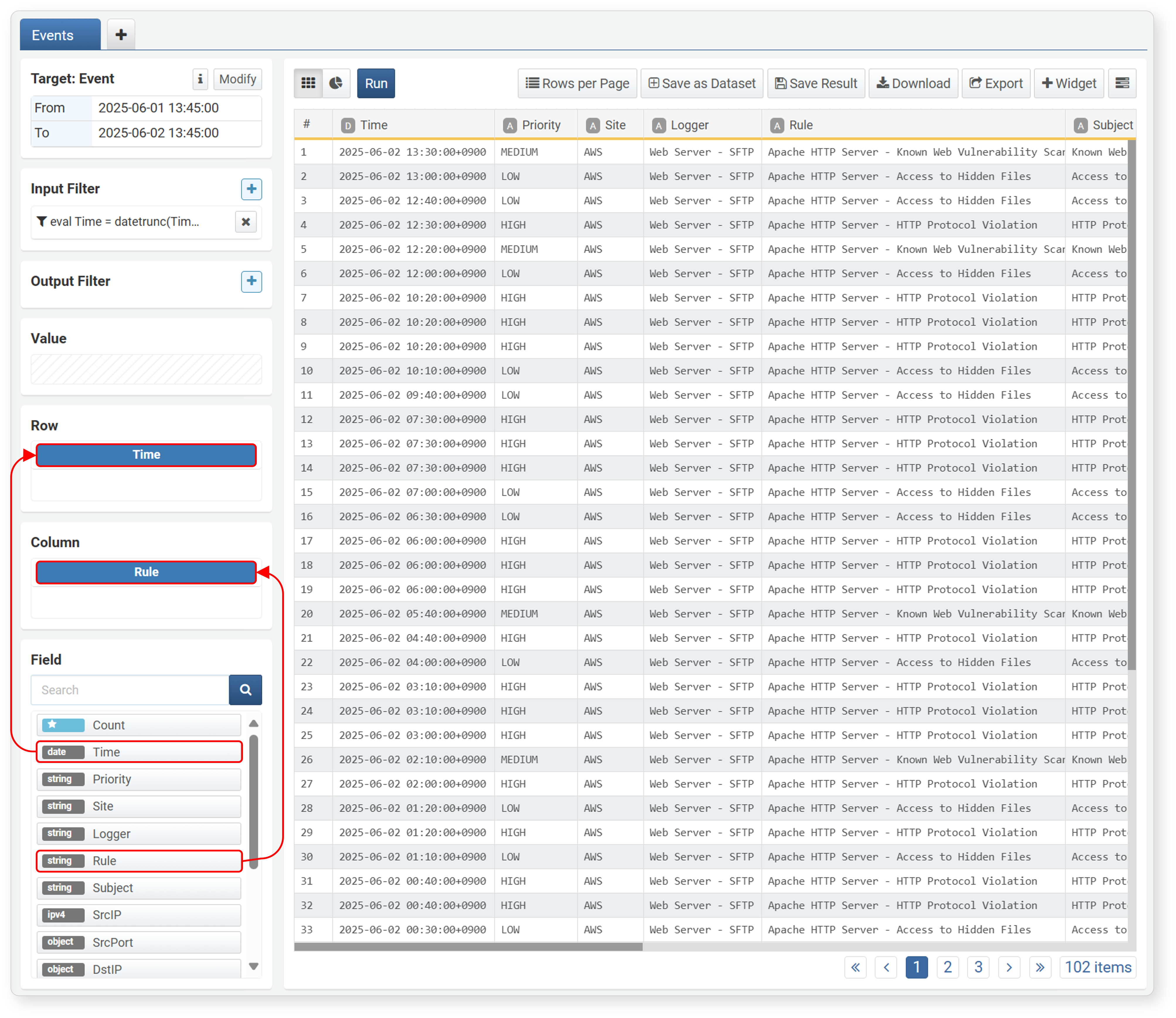
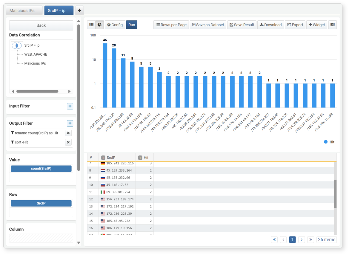
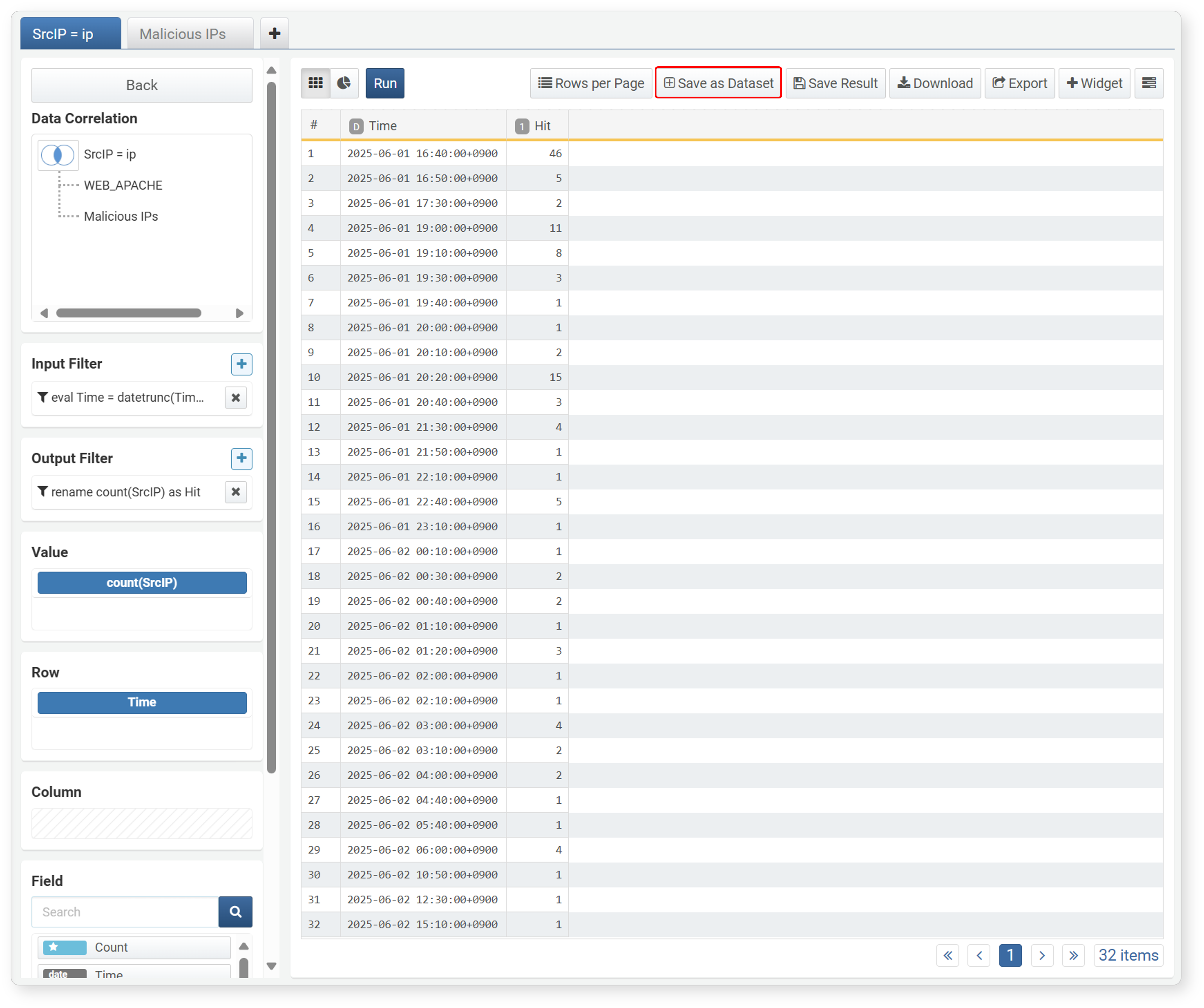
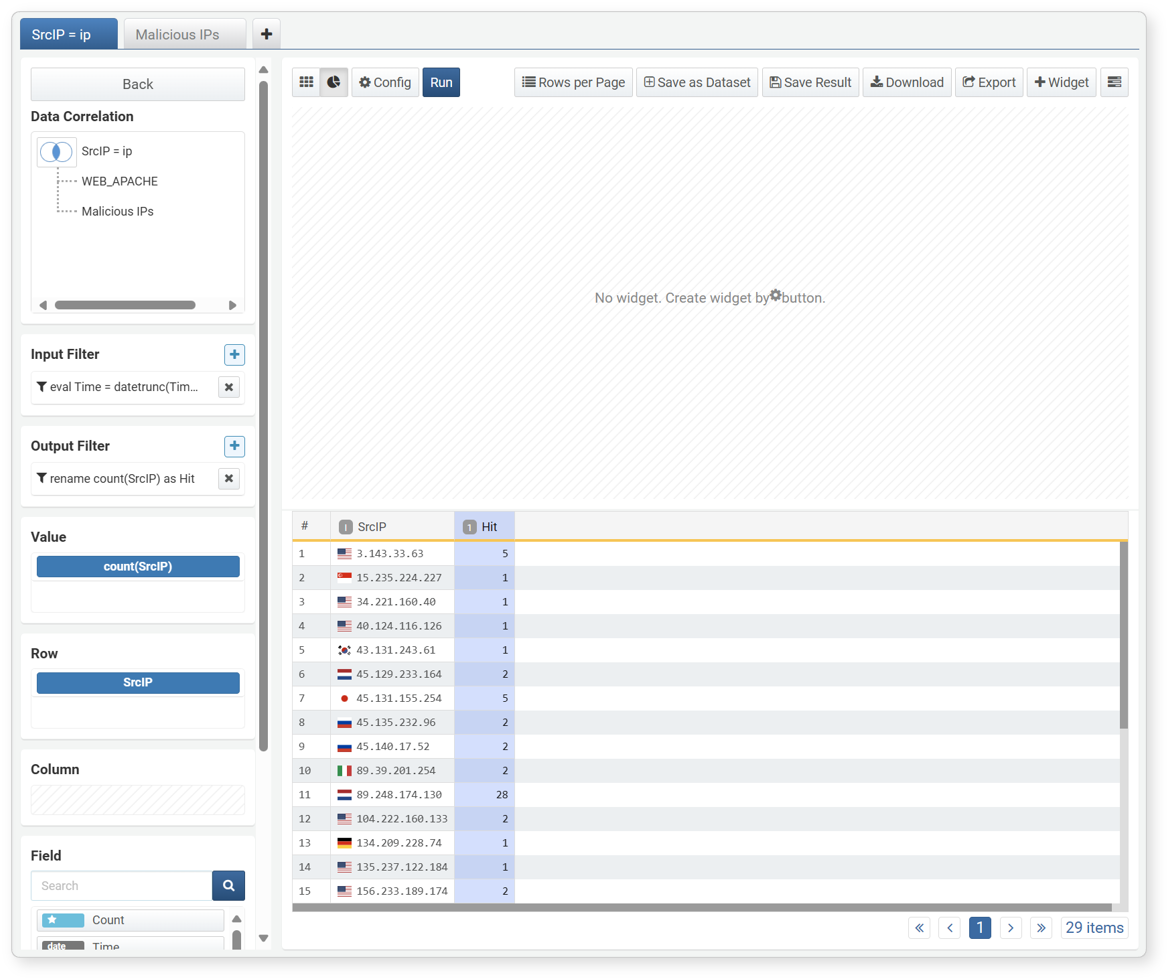
In this example, the attacker IP address is set as the row, and the count of web server logs is set as the value to show the number of attacks per IP address.
- Row: Attacker IP address
- Column: Not specified
- Value: Count of web server logs
- Change Correlation Condition
-
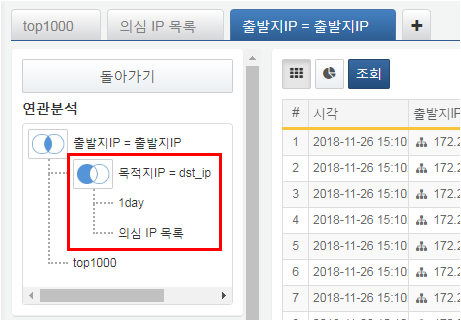
Click the correlation analysis type (diagram icon) on the left of the correlation analysis screen to change the correlation analysis type and correlation fields.
- Other Operations
-
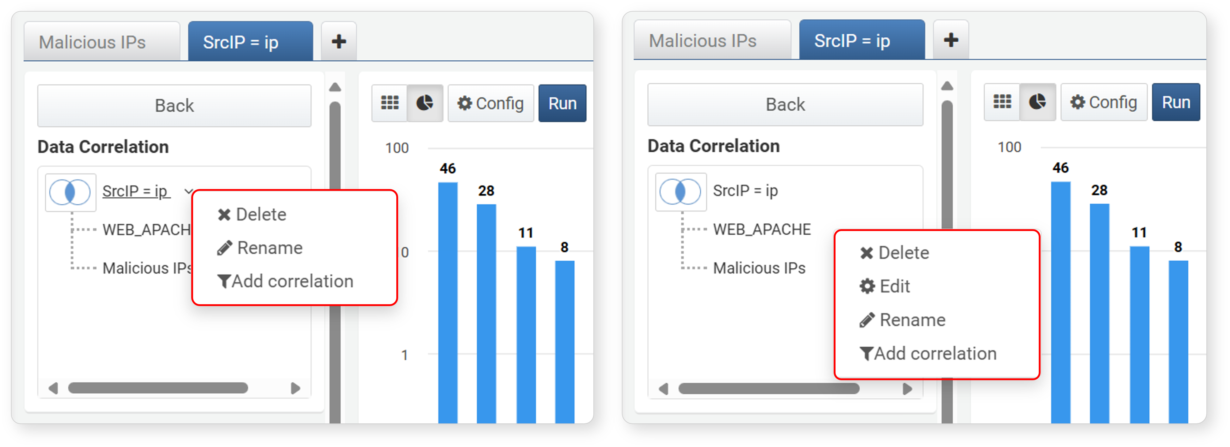
Clicking the correlation analysis name or tab name in the correlation analysis screen brings up a popup menu. You can delete, edit, rename, or add correlation analysis from the popup menu:
- Delete
-
You can delete the selected data group or correlation analysis.
- If you execute Delete at the root of the tree (node with the correlation type diagram), the correlation analysis ends and returns to the previous state.
- If you select a data group in the tree and execute Delete, that data group is removed from the correlation analysis.
- Edit
-
To reconfigure the data group used in the correlation analysis, click Edit. Clicking Edit switches to the edit screen for the selected data group, where you can reload and process the data. You can change the data type, search period, filter settings, aggregation fields, etc. After editing, click Back to return to the correlation analysis screen.
- Rename
-
You can rename the correlation analysis or data tab. Renaming makes it easier to identify data during the process. Enter a new name in the Rename dialog and click Modify to apply the change immediately.
- Add Correlation
-
You can add a new correlation analysis to the data being correlated. Click the column title or correlation analysis name, then select Add Correlation from the popup menu. In the New Data Correlation dialog, set the Selected Tab, Data Correlation Type, Left correlation field, and Right correlation field to configure a new correlation analysis. You can apply additional correlation analysis to an already applied correlation analysis.
-
When you add a correlation analysis, it is displayed as an additional correlation analysis in the correlation analysis screen.
- End Correlation Analysis
-
Click Back in the correlation analysis screen or select Delete from the popup menu after clicking the correlation analysis name to end the correlation analysis. Ending the correlation analysis deletes all filters and aggregation fields set in the correlation analysis screen and returns to the original pivot screen.
Utilizing Analysis Results
The results analyzed in the pivot can be utilized in various ways. You can use the analysis results for other analysis tasks or add them as dashboard widgets for real-time monitoring.
Ways to utilize analysis results include:
- Save the analysis results as a dataset to use as base data shared by multiple dashboard widgets or for pivot analysis
- Convert the analysis results into a dashboard query widget
- Export as a file for use in other systems
- Export as a pivot file for use in other Logpresso Sonar systems
- Save only the analysis results for use in other analyses
Dataset
To save analysis results as a dataset:
-
Prepare the data to be suitable for saving as a dataset.
- Set the range to Recent Period. Datasets should be saved with data specified for a recent period for easier reuse.
- If necessary, remove the default filter Limit results to 10,000 in the output filter. If there is a lot of data collected during the specified period, some data may be omitted.
- If you need to aggregate values, add a time unit truncation expression to the input filter for the Time field. For example, you can add a time unit truncation (unit: 10 minutes) expression to aggregate values in 10-minute intervals.
-
Click Save as Dataset in the toolbar.
-
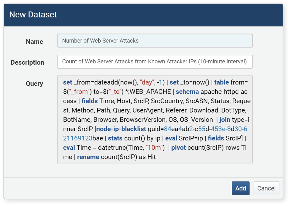
In the Add Dataset dialog, enter the name (up to 50 characters) and description (up to 2,000 characters) of the dataset, then click Add.
-
Check the saved dataset in Analysis > Dataset.
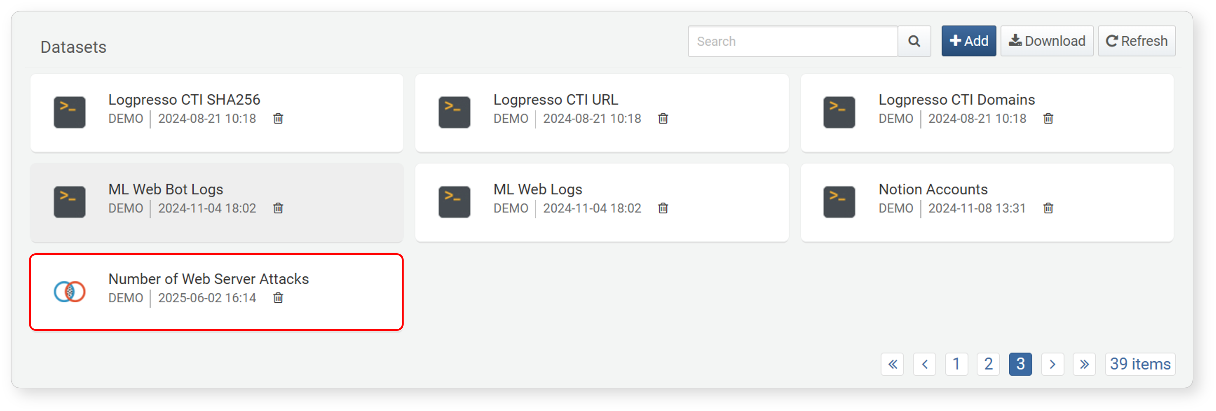
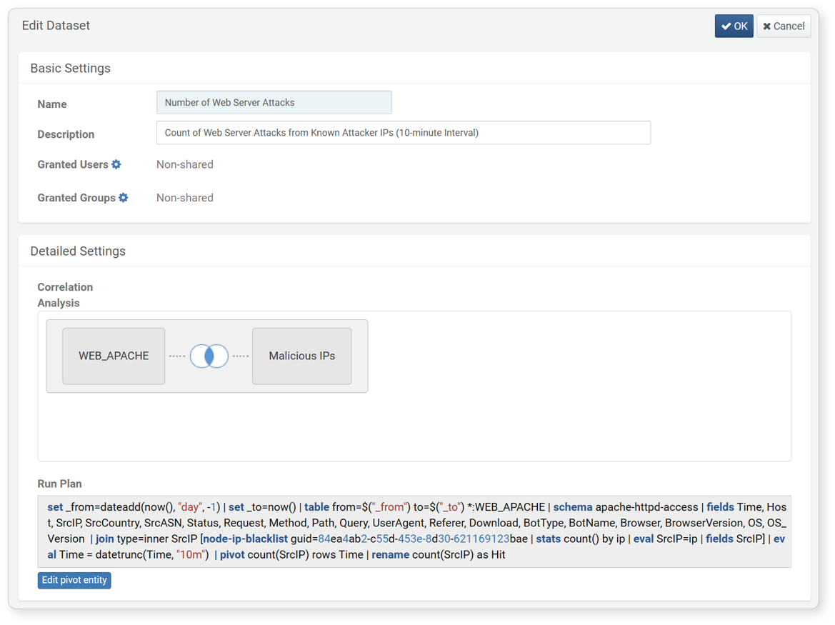
Click the dataset card to view and edit the details.
Widget
A widget is a tool for visualizing data on the dashboard. You can add data analyzed in a pivot table to the dashboard as a chart or grid for real-time monitoring.
Grid
To create a grid widget:
-
Load and process the data as needed.
-
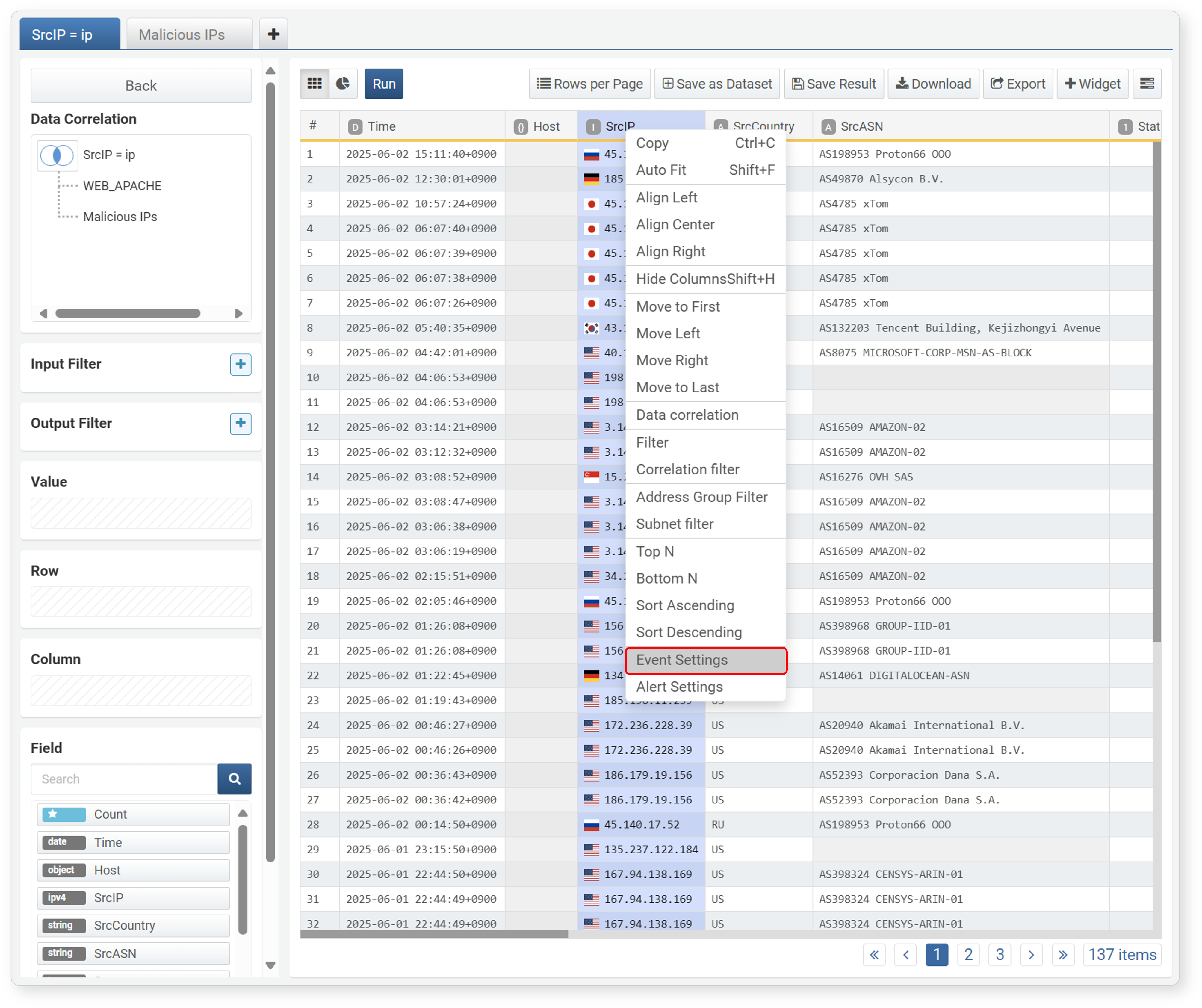
To apply a filter, execute a query, or open a browser when clicking a cell, set an event.
-
To change the cell color and play an alert sound when a specific field value exceeds a threshold, set an alert.
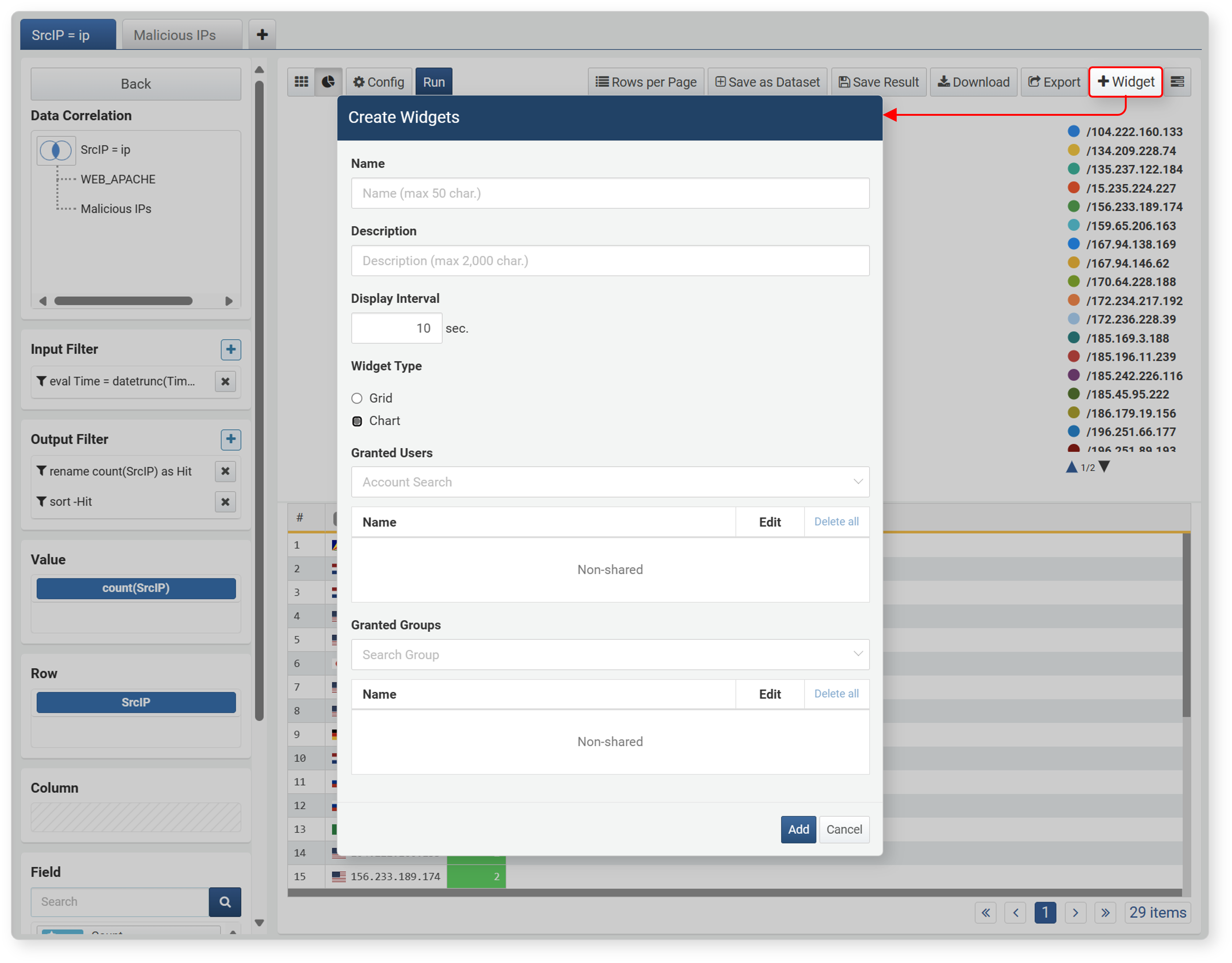
-
In the toolbar, click Widget, then enter/select the required properties in the Create Widget dialog and click Add.
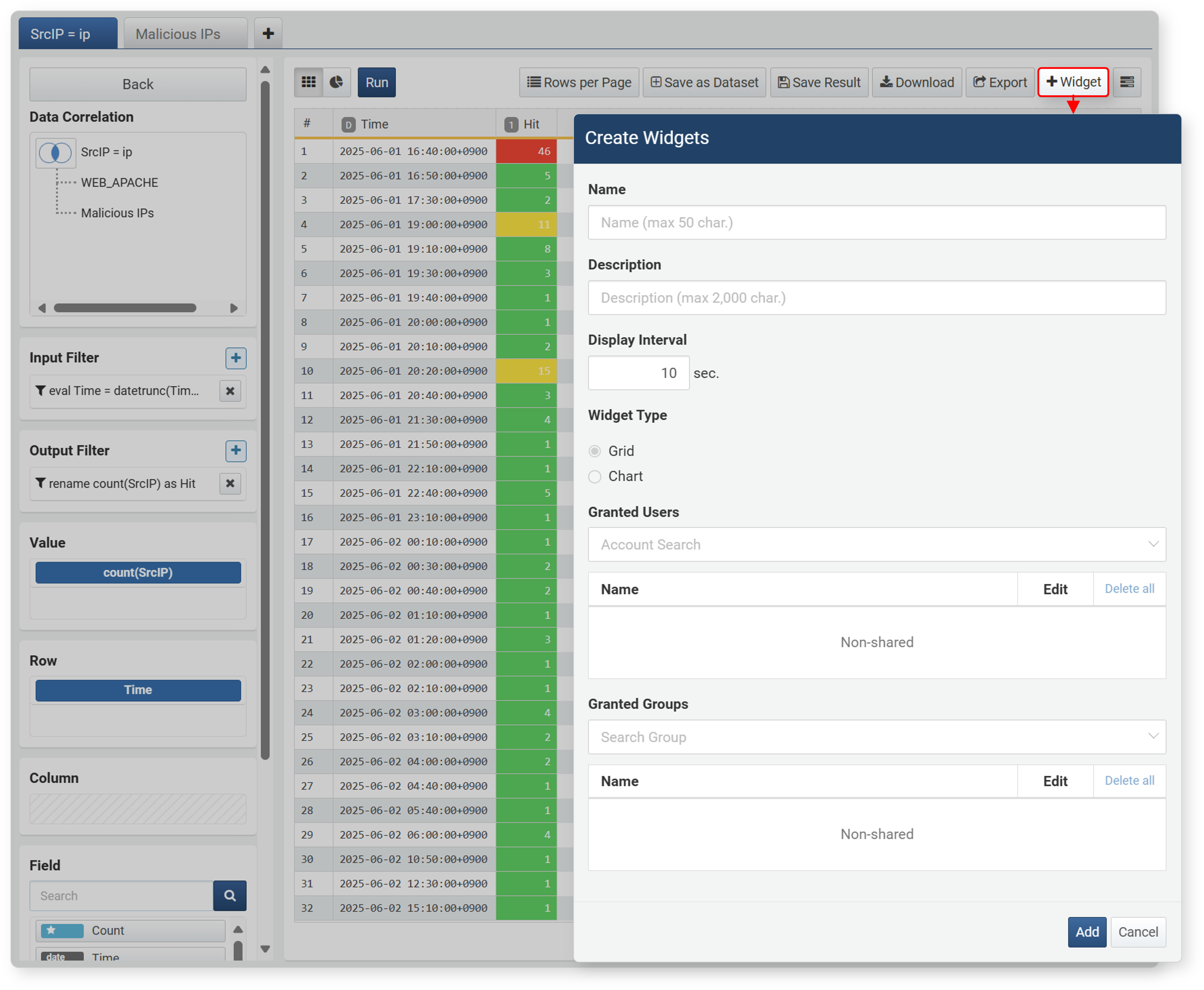
- Name: Unique name of the widget (up to 50 characters)
- Description: Description of the widget (up to 2,000 characters)
- Display Interval: Execution interval of the widget (1~2,147,483 seconds). Set an appropriate value according to the amount of collected data to avoid issues during monitoring. If data needs to be updated quickly, set a short interval, but if there is a lot of data, set an appropriate interval considering performance.
- Widget Type: Type of widget to add (default: grid)
- Granted Users/Groups: Set the account or account group to share the widget with
-
The added widget can be checked in Dashboard > Widget Management.
Chart
To create a chart widget:
-
Prepare the data to be suitable for chart widget representation.
- Data should be in the form of independent and dependent variables.
- Independent variable fields are fields with unique values, such as time, IP address, or user ID.
- Dependent variable fields are fields with aggregate values.
-
In the toolbar, click
 , then Settings in order.
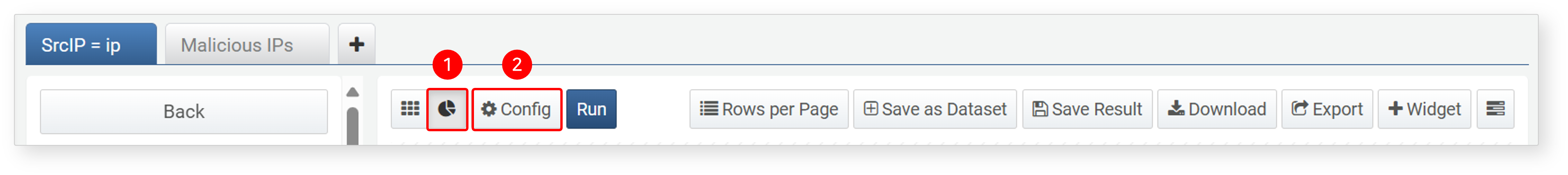
-
When the Widget Settings screen appears, complete the settings and click OK.
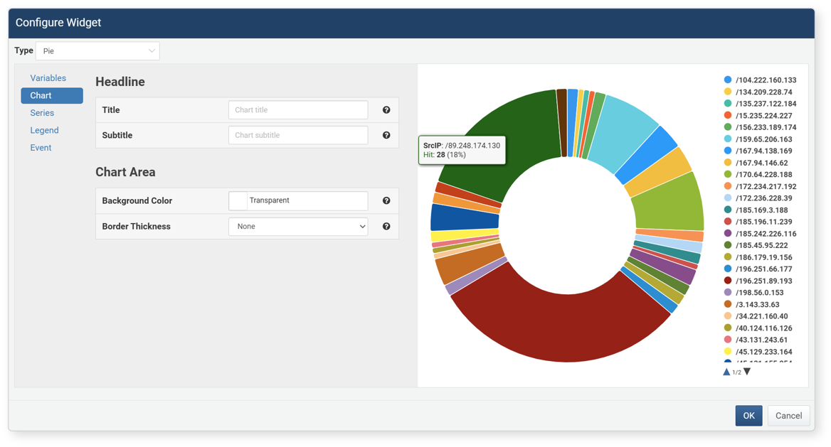
- Type: Chart type. Other properties vary depending on the type (default: line).
- Line: Line time series chart
- Spline: Smooth line time series chart
- Area: Area-filled line chart
- Area (Spline): Area-filled spline chart
- Horizontal Bar: Chart expressing a single dependent variable as a horizontal bar
- Vertical Bar: Chart expressing a single dependent variable as a vertical bar
- Stacked Area: Area chart stacking multiple dependent variables
- Stacked Area (Spline): Stacked area (spline) chart for multiple dependent variables
- Scatter: Chart expressing dependent variable values as points
- Pie: Pie or donut chart
- Stacked Horizontal Bar: Stacked horizontal bar chart for multiple dependent variables
- Stacked Vertical Bar: Stacked vertical bar chart for multiple dependent variables
- Treemap: Chart expressing values with color and area
- Alert Box: Message box that displays color when exceeding a threshold
- World Map (Marker): Chart expressing data with latitude and longitude as markers on a world map
- World Map (Bubble): Chart expressing data with latitude and longitude as bubbles on a world map
- Event: Executes a specified action when clicking or dragging a component in the chart. For details, see Event Settings.
- Type: Chart type. Other properties vary depending on the type (default: line).
-
In the toolbar, click Widget, then enter/select the required properties in the Create Widget dialog and click Add.
- Name: Unique name of the widget (up to 50 characters)
- Description: Description of the widget (up to 2,000 characters)
- Execution Interval: Execution interval of the widget (1~2,147,483 seconds). Set an appropriate value according to the amount of collected data to avoid issues during monitoring. If data needs to be updated quickly, set a short interval, but if there is a lot of data, set an appropriate interval considering performance.
- Widget Type: Type of widget to add (default: chart)
- Account Sharing/Group Sharing: Set the account or account group to share the widget with
-
The added widget can be checked in Dashboard > Widget Management.
Event Settings
When you click a cell in a grid widget or click or drag a visual element in a chart widget, you can specify the action to perform.
The setting method is the same for both grid and chart widgets. The settings for each action are as follows.
- Apply Filter
- Applies a filter to the entire dashboard or dataset. You can add one or more filters.
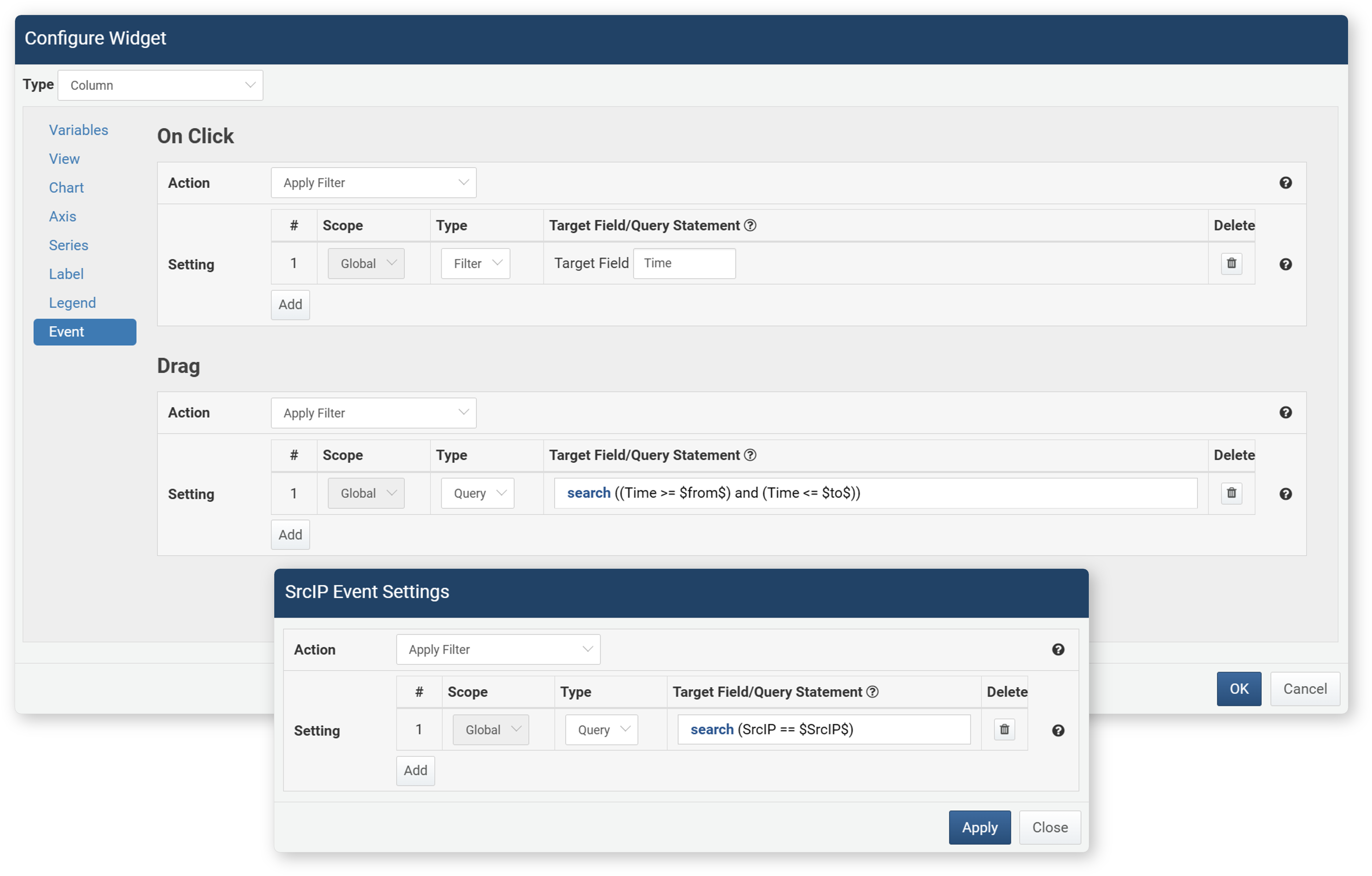
- Scope: The scope to apply the filter to (Global: the entire dashboard containing the widget, Dataset: the dataset being viewed). Only Global is supported in widgets.
- Type (default: Filter)
- Filter: Shows only values matching the target field.
- Query: You can directly enter a query.
- Target Field/Query: Enter the target field or query
- Delete: Click the
 icon to delete the added filter
The following macros can be used in queries.
Macro Description Widget Type Event $FieldName$Field value Grid, Chart On click $x$Independent variable value Chart Click $xfield$Independent variable field name Chart On click, Drag $from$Start value of period Chart Drag $to$End value of period Chart Drag - Run Query
- Opens a new query window and executes the user-specified query.
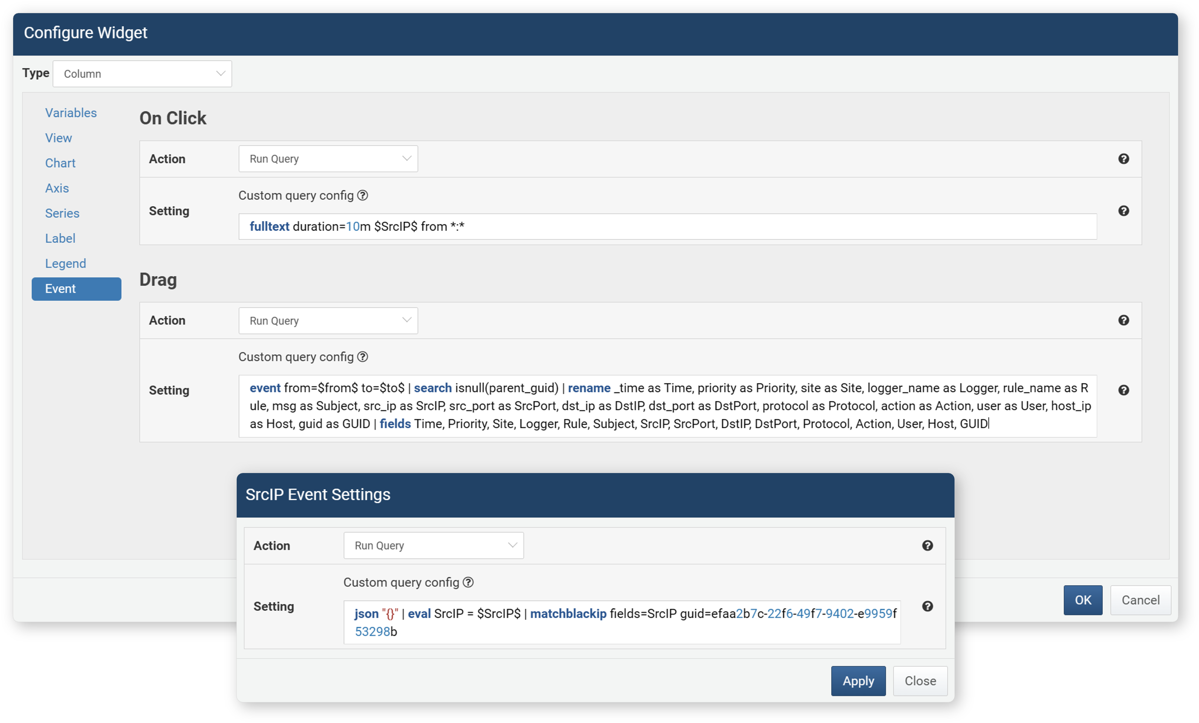
The query entered in Settings must start with a data retrieval command (driver query command). The queries in the figure above start with commands such as fulltext, event, or json.
The following macros can be used in queries.
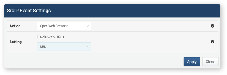
Macro Description Widget Type Event $FieldName$Field value Grid, Chart Click $series$(Dependent variable) field name Grid, Chart Click $xfield$Independent variable field name Chart Click, Drag $from$Start value of period Chart Drag $to$End value of period Chart Drag - Open Web Browser
- Opens a new window in the web browser and accesses the URL in the specified field. Drag events are not supported for opening the browser.
- Navigate to ...
- Switches the screen to the specified URL in the connected web console window. Drag events are not supported for screen transitions.
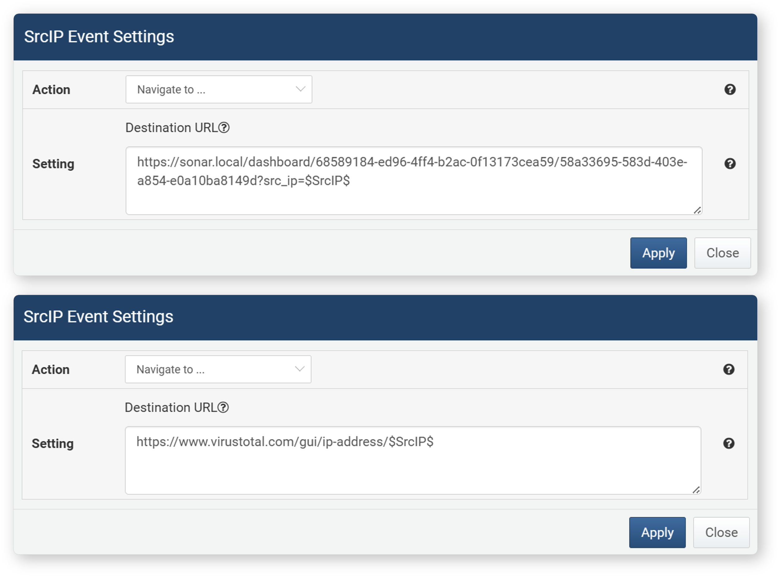
The following macros can be used in the screen transition URL.
Macro Description Widget Type Event $FieldName$Field value Grid, Chart Click $series$(Dependent variable) field name Grid, Chart Click
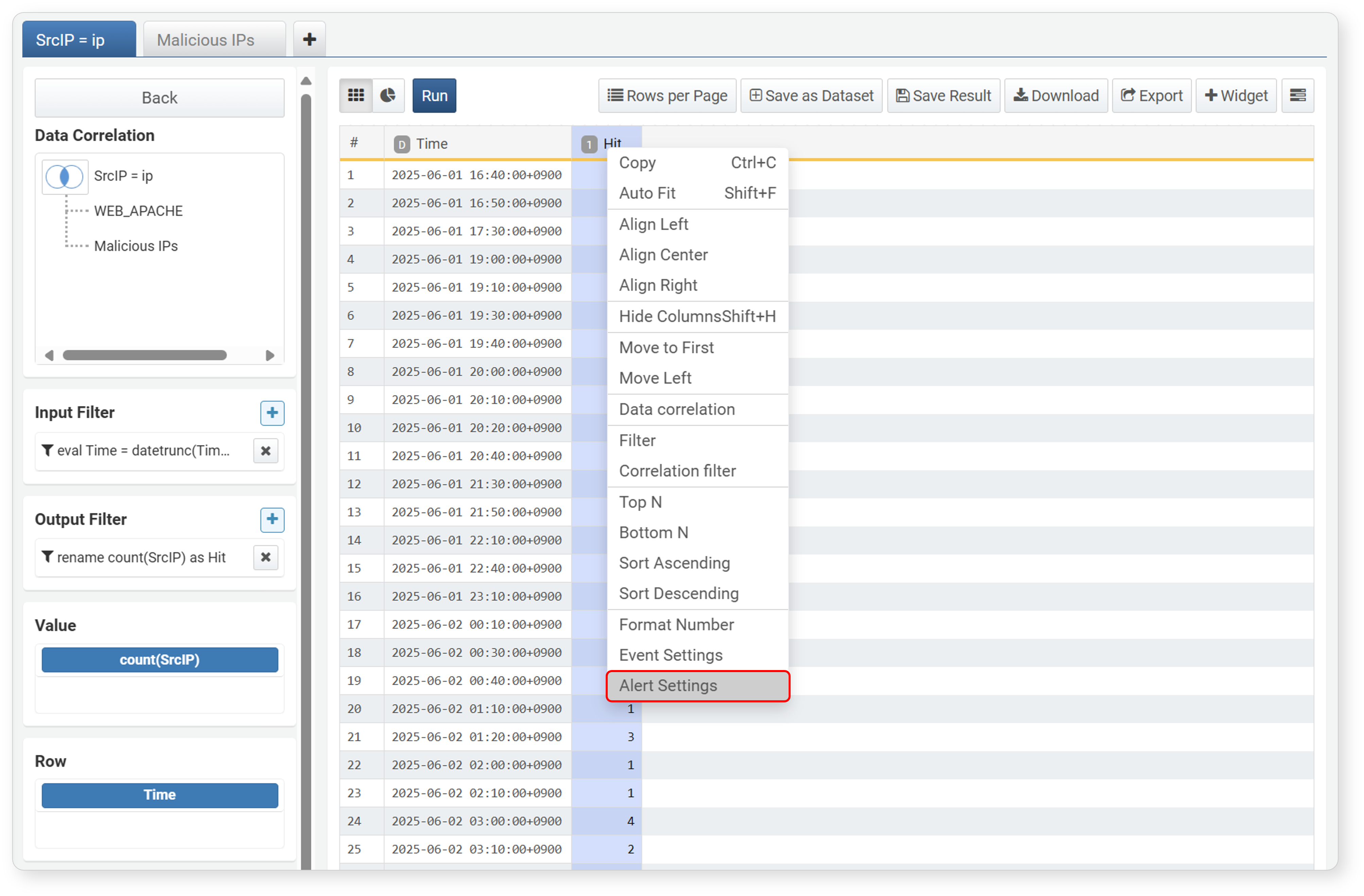
Alert Settings
This feature triggers an alert when a specific field value in a grid widget exceeds a threshold. Alerts are displayed as a notification message at the bottom right of the browser with a sound. Setting alerts allows you to monitor data in real time on the dashboard.
To set an alert, right-click the field name in the grid edit screen and click Alert Settings in the popup menu.
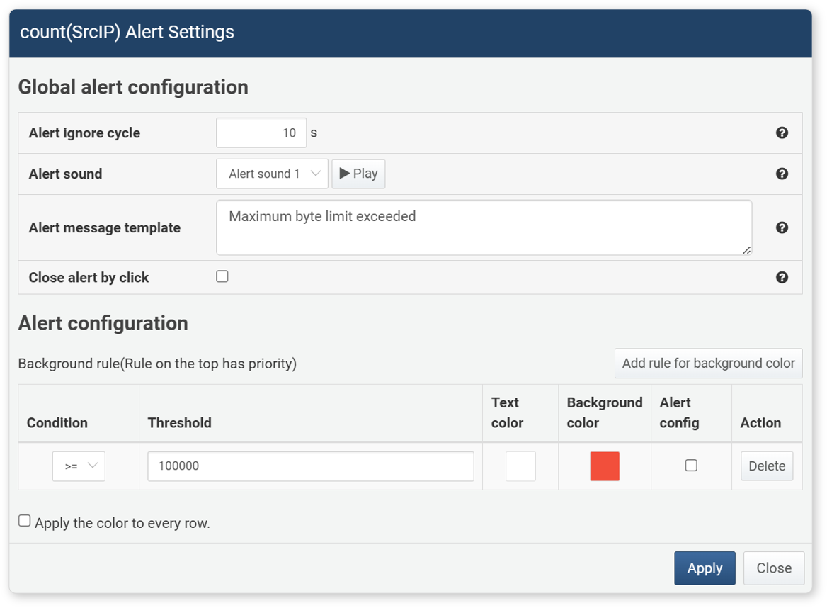
The following items can be set in the Alert Settings dialog.
-
Alert Ignore Cycle: After an alert occurs, no alert is triggered for the specified time (1~2,147,483 seconds, default: 10 seconds)
-
Alert Sound: The sound to play when an alert occurs
-
Alert Message Template: The message to display when an alert occurs (up to 5,000 characters). You can use the following macros to create a custom alert message.
Macro Description $FieldName$Field value displayed in the grid $rulefield$Alert target field name $rulevalue$Alert target field value $ruleoperators$Condition operator ( ==,!=,>,>=,<,<=)$ruleoperands$Threshold -
Click Alert by Click: Allows the user to manually close the alert notification message displayed at the bottom right of the browser (default: disabled).
-
Background Rule: Alerts are triggered in the order registered, with the top condition having the highest priority.
- Condition: The condition to compare with the field value for the alert
- Threshold: The reference value for evaluating the alert condition. If the selected field value meets the condition with this threshold, an alert is triggered.
- Text Color: Text color when the condition is met
- Background Color: Cell background color when the condition is met
- Alert Config: Set to play an alert sound or display an alert message when the condition is met
- Action: Click Delete to remove the added alert condition
-
Apply color to every row: Set this option to apply the alert color not only to the selected field but also to all cells in the row.
Save Query Results
To save analysis results as query results:
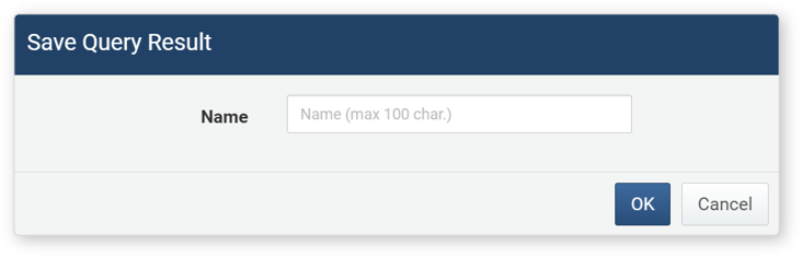
- In the analysis search result screen, click Save Query Results in the toolbar.
- In the Save Query Results dialog, enter the name to save and click OK.
-
Query result data is saved on the server and can be checked in Analysis > Query under Load Query Results. For details, see Load Query Results.
-
Export as Pivot File
You can export analysis results as a pivot file to your local PC. Click Export in the toolbar, enter the file name (letters, numbers, special character '_') in the Export Pivot dialog, and click Export.
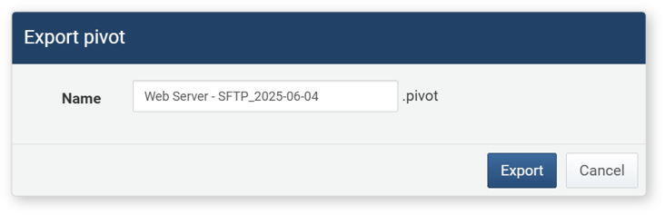
Exported pivot files can be viewed again using the Import function.
Download
To save analysis results to your local PC, click Download in the toolbar. In the Download Query Results window, enter or select the properties of the analysis results, then click Download.
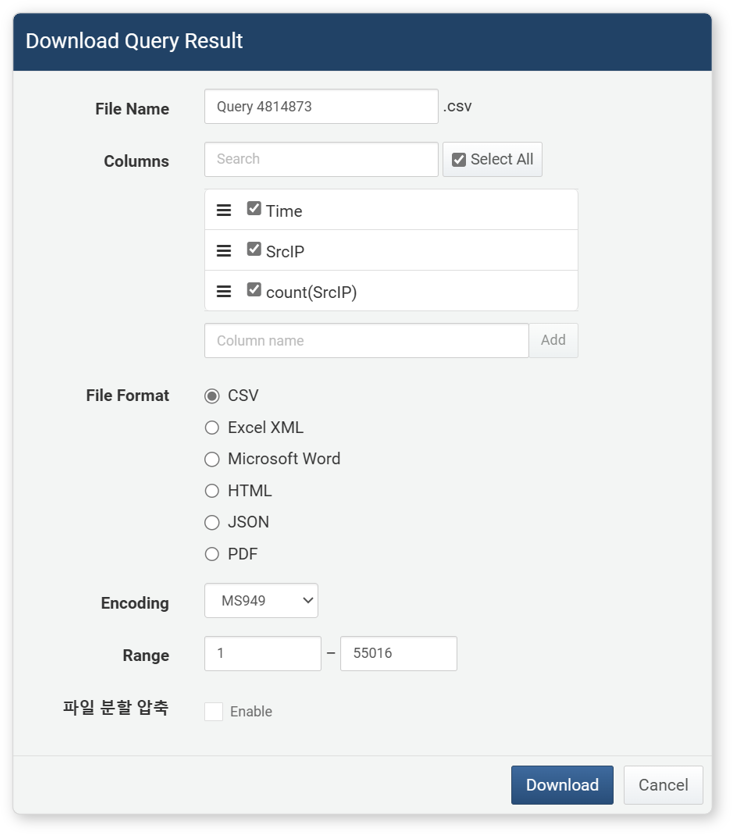
- File Name: Name of the analysis result file to download (default: ticket)
- Columns: Properties of the analysis results to save in the file. Click Select All to record all properties in the file.
- File Format: Format of the file to download (default: CSV)
- CSV: CSV file
- Excel XML: XML file viewable in Microsoft Excel
- Microsoft Word: DOCX file
- HTML: HTML file
- JSON: JSON file
- PDF: PDF file
- File Encoding: File encoding (UTF-8, UTF-18 BE, Extended Wansung, default: Extended Wansung)
- Range: Number of analysis results to record in the file. Only the specified number of most recent analysis results are recorded in reverse chronological order.
- Split and Compress File: Used to save analysis results by splitting into multiple files (default: disabled). If enabled, files are split and compressed in units of 100,000 records (can be changed).
Set Number of Analysis Data to Display
The analysis data list is paginated in units of 50 records. To change the number of data displayed per page, click Display Count in the toolbar of the analysis result screen and change the setting.
View Analysis Query Execution Information
You can check the query used for the current pivot condition, the time the query was executed, the query duration, and the number of records at each stage. Click the  icon in the toolbar to display the information at the bottom of the screen.
Import Pivot
If you have exported the settings of a previously executed pivot query, you can import those settings to run the pivot again. To import a pivot:
-
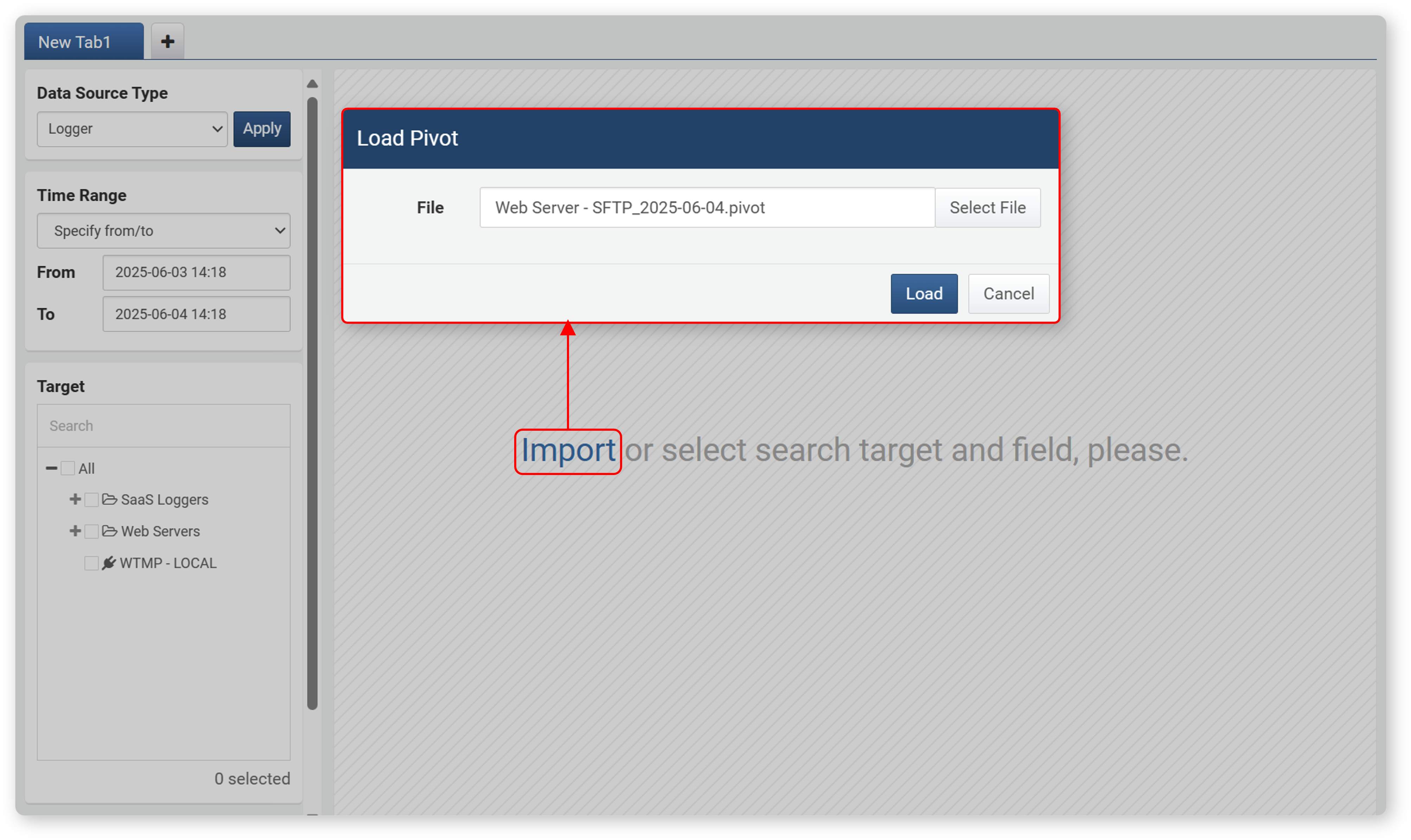
In Analysis > Pivot, click Import in the center of the screen.
-
In the Import Pivot dialog, click Select File, select the file saved in .pivot format, and click Import.
-
The query is executed based on the time the pivot was imported, and data is retrieved. For example, if the data retrieval period is set to the last 1 day, the most recent 1 day's data is retrieved at the time of import.
If an error occurs when importing a pivot, refer to the following:
- The logger, behavior profile, or dataset at the time of export does not exist
- The table with the same name as at the time of export does not exist
- If some loggers or tables at the time of export do not exist, only partial import is performed
- If the user account performing the import does not have permission for the data source in the pivot file
- If the pivot file is corrupted
- If the file extension is not .pivot