Pivots
Overview
Use Analysis > Pivots to group and aggregate collected logs, events, datasets, and behavior profile results by item and analyze relationships and distributions. While the Logs page is better suited for reviewing individual records directly, the Pivots page is better for summarizing and comparing the same data to quickly identify recurring patterns or anomalies.
SOC analysts typically use pivots in the following situations:
- Analyzing distributions: Aggregate web access logs by bot type or by IP range to compare the distribution of normal traffic with suspicious traffic.
- Cross-checking indicators: Split the analysis across multiple tabs so that event logs and threat intelligence data are loaded separately, then run a correlation analysis to check whether indicators appear in the internal logs.
- Automating periodic reports: Save recurring aggregations as widgets so that dashboards refresh them automatically for continuous monitoring.
Analysis results created in Pivots can be saved as a dataset for reuse as the base data for other analyses, or added as a widget to be monitored continuously on a dashboard. Frequently used data source conditions and field layouts can be exported as a .pivot file so the same analysis setup can be reproduced quickly.
Account permissions
| Feature | Administrator (Master, Administrator) | User |
|---|---|---|
| Access the Pivots page | ✔ | ✔ |
| Download query result | ✔ | ✔ |
| Save query result | ✔ | ✔ |
| Save as dataset | ✔ | ✔ |
| Export and import pivot files | ✔ | ✔ |
| Add widget | ✔ | — |
The Pivots page requires the pivot view permission, which is granted to user accounts by default. Even with this feature permission, you can only load data from tables you have access to.
Only accounts with the dashboard management or widget edit permission can add widgets.
Workflow
The following diagram illustrates the overall process of analyzing data with pivots.
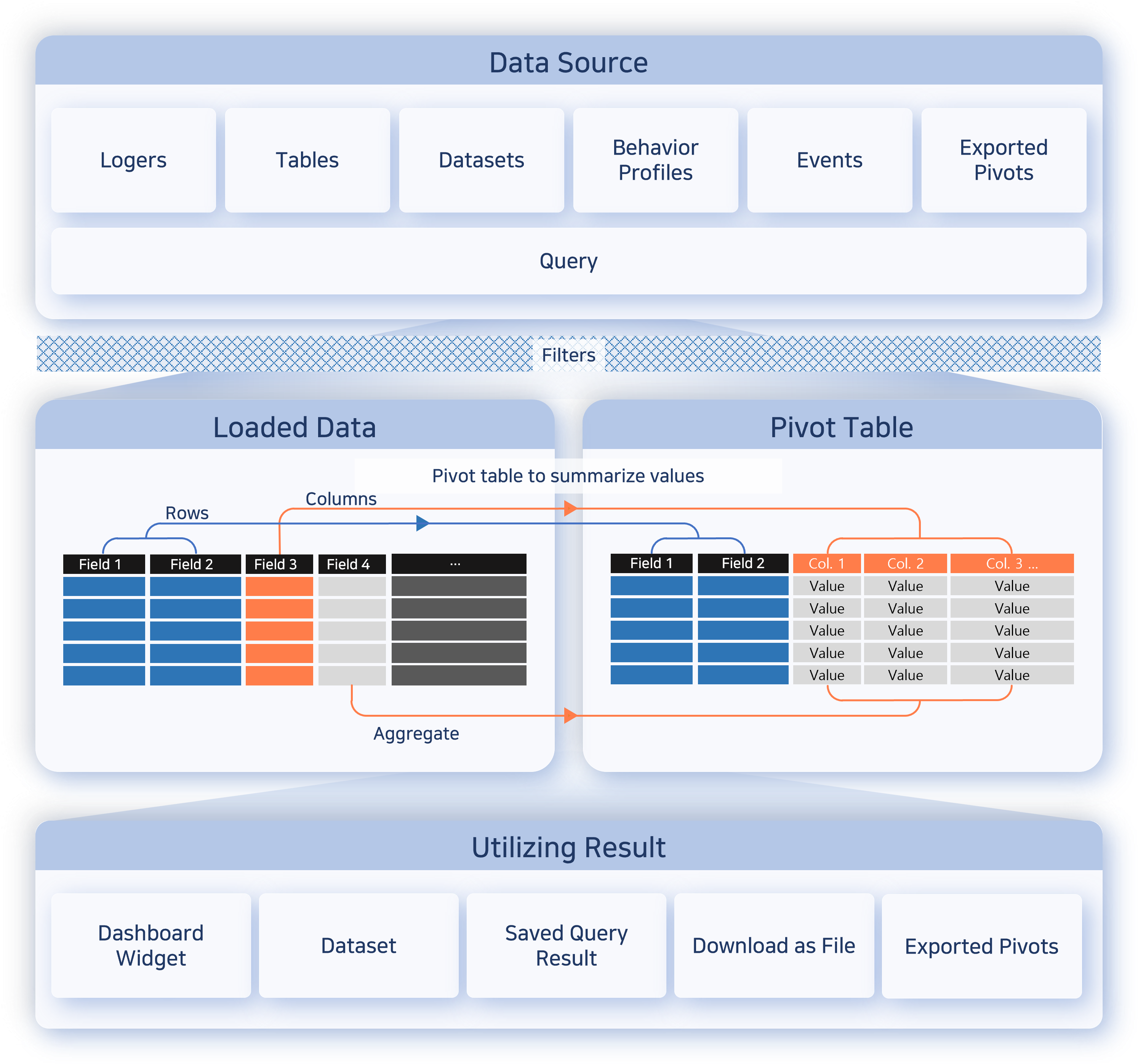
- Step 1: Load data
- Load the target data into the workspace by specifying Data Type, Range, Target, and Schema.
- Step 2: Process data
- Use input filters, result filters, field organization, and value/row/column placement to shape the data into a form suitable for analysis.
- Step 3: Analyze data
- Use the pivot table or correlation analysis to compare relationships between items and review distributions and aggregated results.
- Step 4: Reuse results
- Save the finished result as a dataset, widget, or pivot file so you can reuse it for repeated analysis or dashboard configuration.
Screen layout
The Pivot screen is divided into a left panel (data-loading tools or analysis tools) and a right workspace. Drag the border between the left panel and the workspace to adjust the sidebar width, or drag it far enough to the left to minimize the panel. This is useful when the panel feels cramped due to many analysis options, or when you want to expand the result grid.
Tabs
Pivots are managed per tab, so you can separate analyses. Click the + button in the upper-right area to open a new tab and run a different analysis alongside the existing one without losing the previous result. Separate tabs are also useful for comparing two data sets in a correlation analysis.

By default, a tab name is the name of the loaded target. When you work with multiple tabs, rename them to match the purpose of each analysis so they are easier to tell apart.
Before loading data
When you first open Analysis > Pivots, the page shows a data loading panel on the left and an empty workspace on the right.
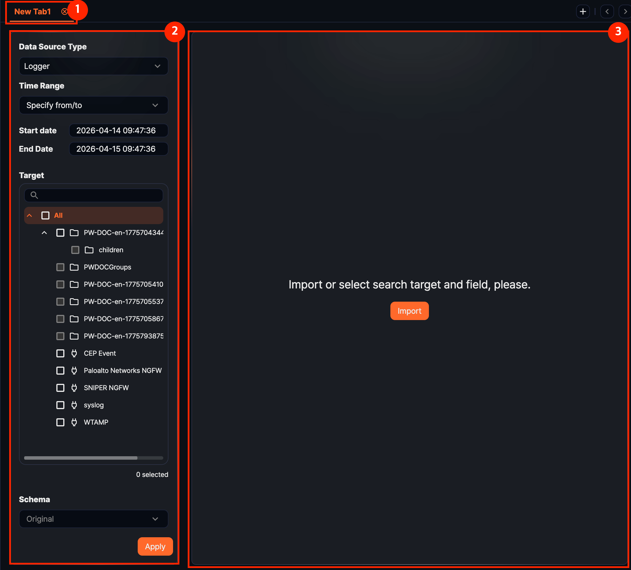
- 1. Tabs
- Pivot work is handled per tab. Open new tabs to run multiple analyses side by side with different conditions.
- 2. Data loading panel
- Use this area to choose Data Type, Range, Target, and Schema and load data into the workspace.
- 3. Workspace
- Before data is loaded, only a guidance message is shown. The result appears after you click Apply. If you have saved a
.pivotfile, you can also click Import Pivot to restore the analysis setup.
After loading data
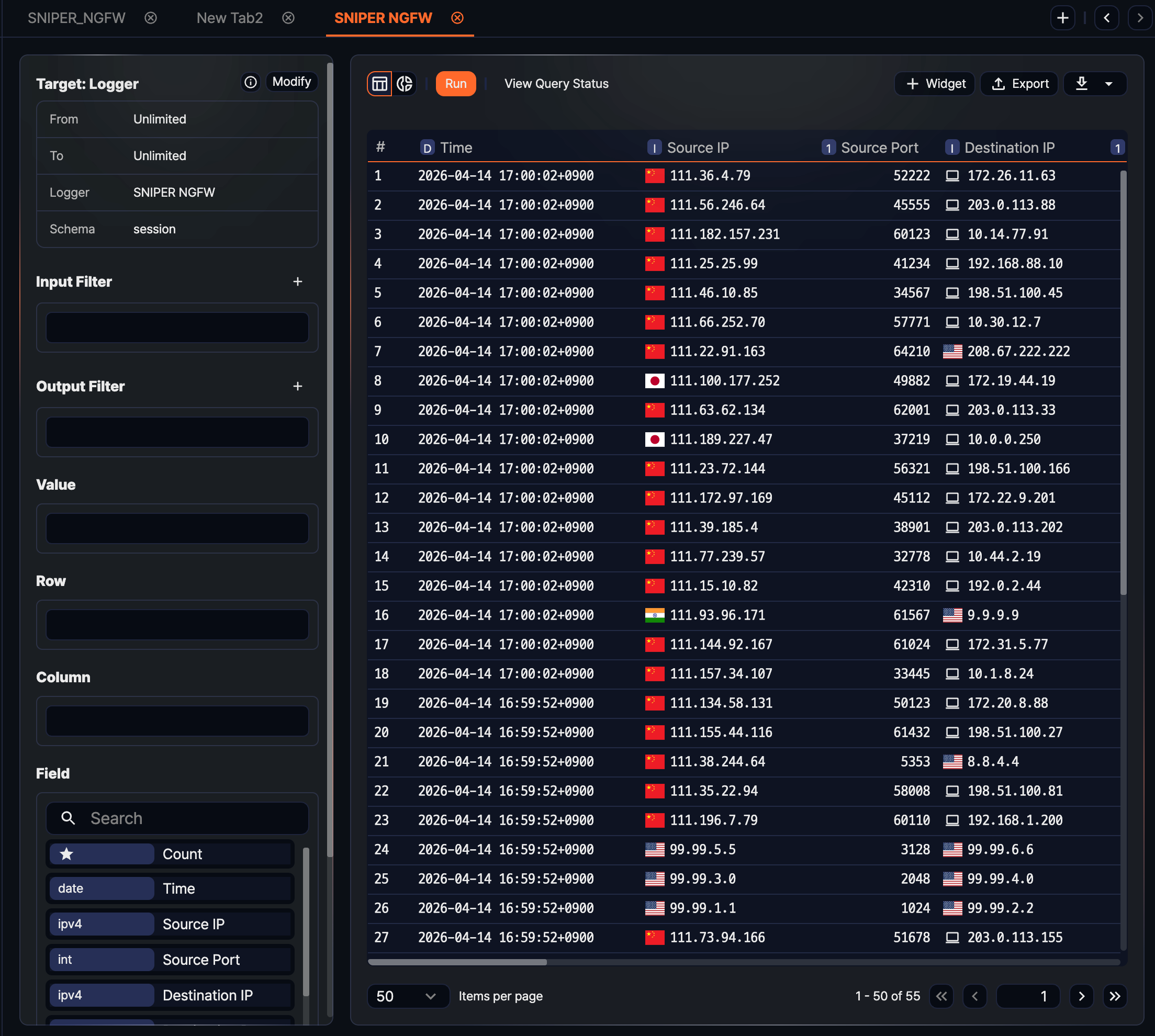
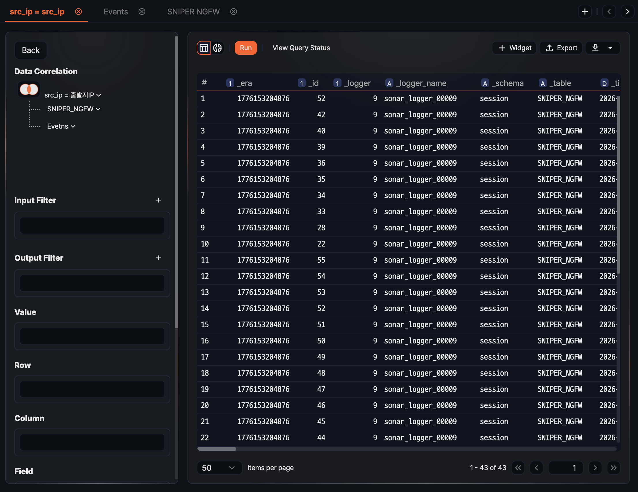
After data is loaded, the tab name changes to the selected target name, and the left panel switches to the analysis-tool layout.
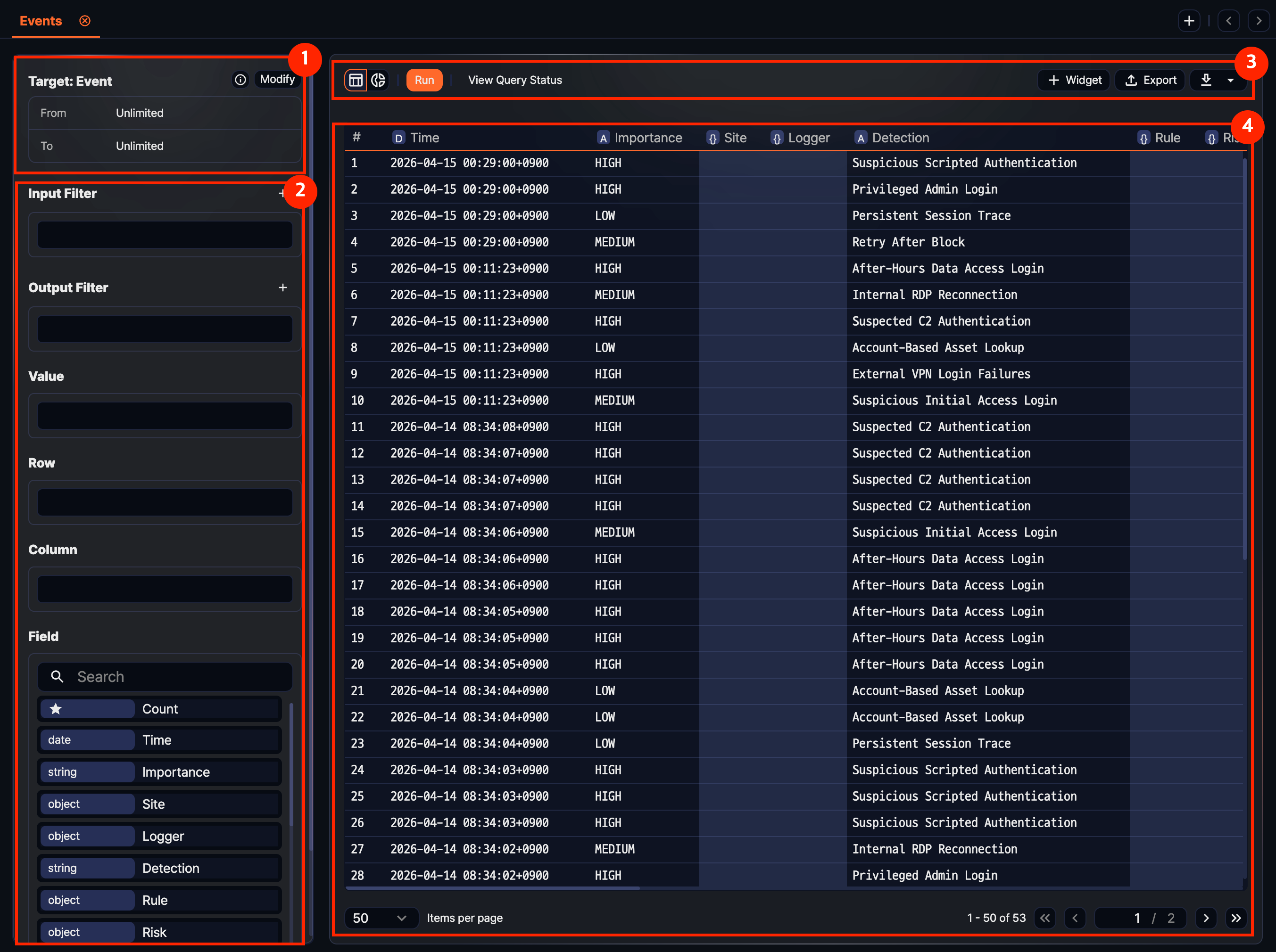
- 1. Query information
- Review the selected Target, Range, Table, and Schema. Click the information area to copy the actual executed query, or click Edit to change the conditions and reload.
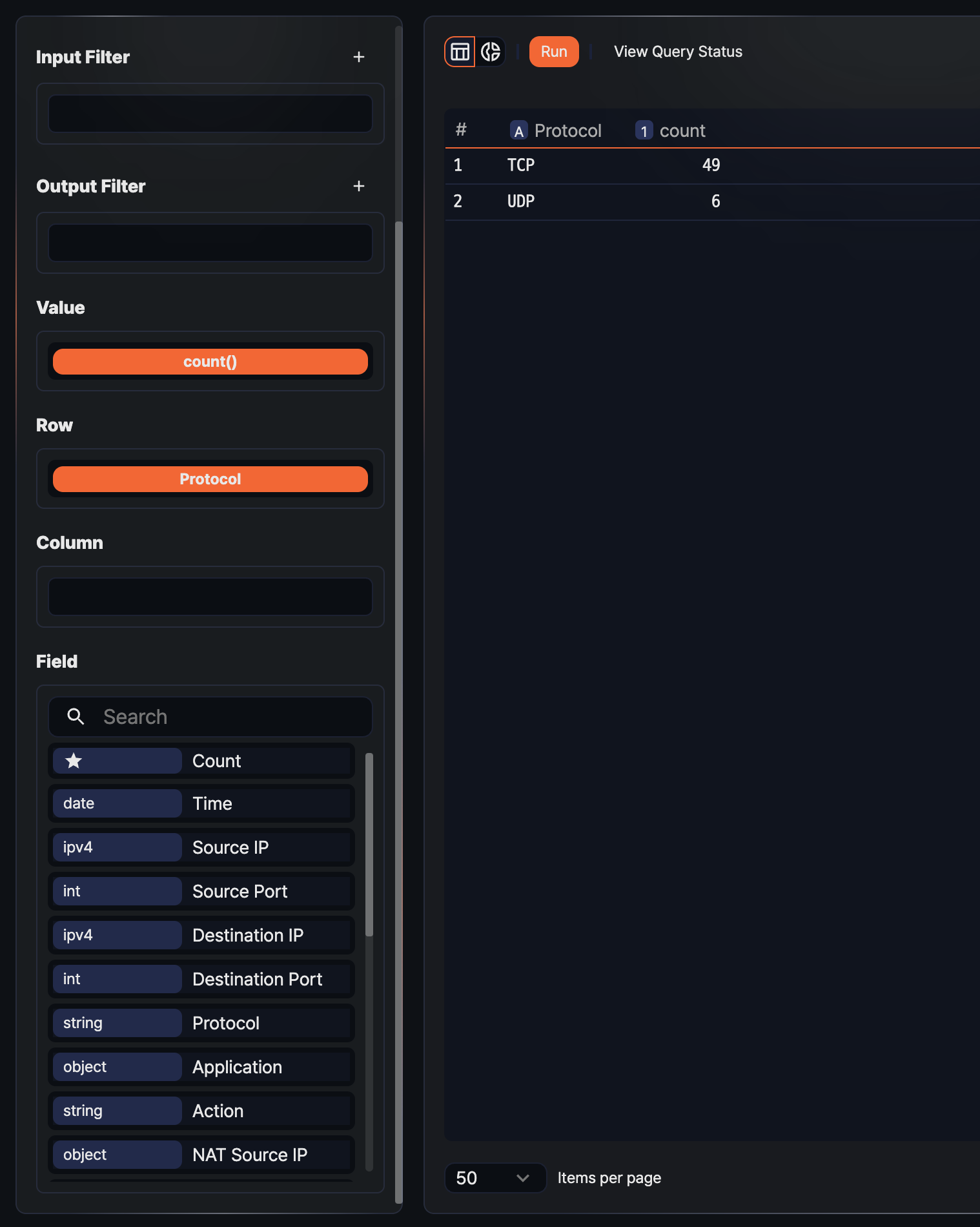
- 2. Analysis tools
- The panel shows Input Filter, Result Filter, Values, Rows, Columns, and Fields. Place fields or add conditions to reshape the result.
- 3. Toolbar
- This area contains follow-up actions such as Run, View Query Status, Widget, and Export. To save the current result as a dataset or download it, click the additional menu button on the right of the toolbar.
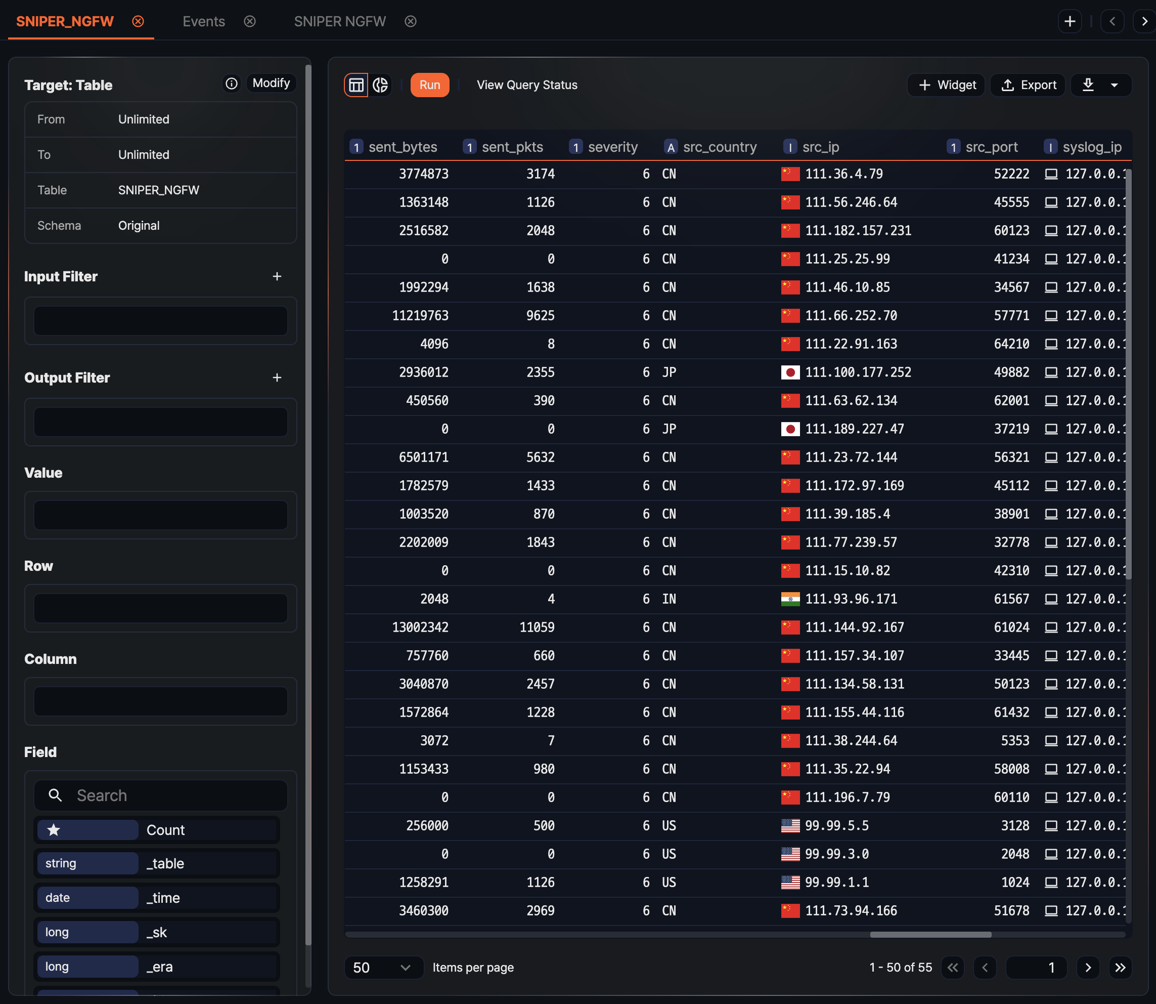
- 4. Result grid
- The loaded data is shown in a table. If no field has been placed into Values, Rows, or Columns yet, the original records appear in grid form first. Use the view toggle above the grid to switch to Chart mode.
Loading data
Specify Data Type, Range, Target, and Schema and click Apply to load data into the workspace. The loaded data becomes the input for the subsequent processing stages such as field selection, filtering, and aggregation. By default, up to 10,000 records are loaded; you can change this limit through the result filter.
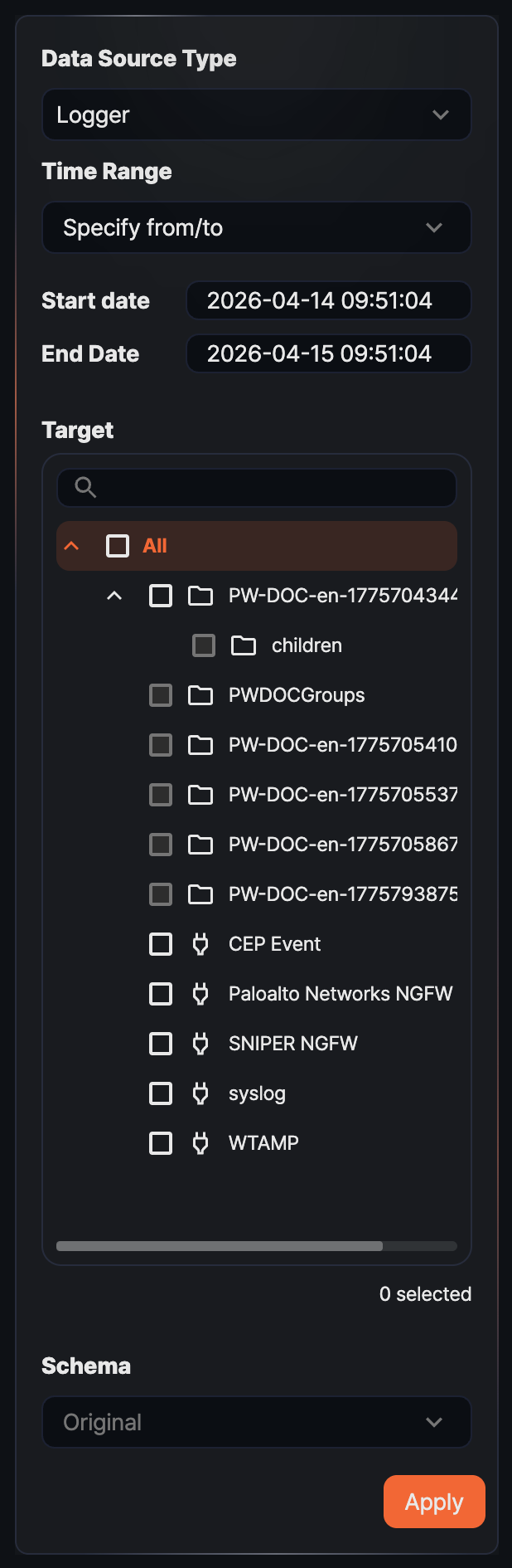
Data Type
Choose the source type of the data to load (default: Logger). The items shown for Target, Schema, and Range depend on the selected type.
- Logger: Loads data collected through the selected logger. If a single table is shared by multiple loggers, only the data loaded through the selected logger is queried.
- Table: Loads data stored in the selected table. Use this option to directly inspect a common table written to by multiple loggers or a system table.
- Dataset: Runs the selected dataset and loads its result. Because a dataset runs a fixed query, Range and Schema cannot be specified.
- Behavior profile: Loads the most recently built data from the selected behavior profile. Use this option to detect anomalies by checking deviations from user and entity behavior.
- Event: Loads event data generated by stream rules or batch rules. Because the event schema is fixed, you do not select a Target or Schema.
- Query: Runs a query you write directly. Use this option when you need a condition that cannot be expressed with the predefined types.
Range
Range specifies the time period to query against the _time field. The range condition cannot be set when Data Type is Dataset or Query. The default is the last 24 hours from the current time, except for Behavior profile, whose default is All time.
- Date range: Queries data between the specified from and to times. The to time is not included in the range.
- Recent: Queries data from the specified from point to the current time (default: 1 day).
- Truncation unit: Truncates the
_timefield value to the selected unit (second, minute, hour, day). The default is no selection. Because the effect is identical to applying the datetrunc() function, it is useful for preparing data at equal intervals for a statistics widget.
- Truncation unit: Truncates the
- All time: Queries every record stored in the selected target.
Target
From the source list that matches the Data Type, select one or more targets to query. For Logger and Table, use a tree with group hierarchy that can be filtered by search terms; the number of selected items is shown below the list. For Behavior profile and Dataset, choose a single item from a dropdown. For Event and Query, no separate target is selected.
Schema
You can specify a schema when Data Type is Logger or Table. When a schema is specified, the original fields are normalized to the schema's field names as they are loaded, and fields not defined in the schema are excluded. The schema dropdown supports search input, so you can find a schema quickly with a partial name match.
- Logger: Choose a schema that matches the normalization rules of the logger model referenced by the selected logger, or Original.
- Table: A table is not bound to a particular schema, so you can choose any log schema registered on the system or Original. Choose the schema that was applied when the data was written to the table.
- Original: Loads the original fields as collected, without normalization. In this case, the field list below is not shown.
Running the load
After you finish setting the conditions, click Apply to load data into the workspace. Once loading finishes, the left option panel switches to the items needed for data processing (filter, value, row, column), and the result table appears in the main area. If you click Apply without filling in all the conditions, an error message appears on the missing items and the load does not proceed. When Data Type is Query, you can also apply by pressing Ctrl + Enter.
Reloading
To load data with different conditions, click Edit on the right of the query information area. The data loading screen opens again with the current conditions pre-filled, so you can change only the parts you need and click Apply. If you change the data type itself, the target and schema are reset. To return without changing anything, click Cancel.
Checking the data source
To see which query was used to load the current data, click the information icon on the right of the query information area. A popover shows the actual executed query so you can see how a logger-based or table-based setup is translated into a query internally.
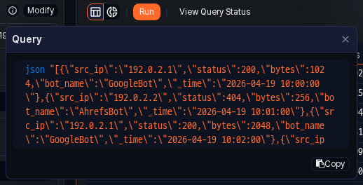
- Copy: Click Copy in the popover to copy the query to the clipboard. Paste the copied query into the Queries page to run it as is, or refine the conditions further and reuse it through the Query type in Pivots.
- Edit: The Edit button next to the popover has the same effect as returning to the data loading screen to change the conditions and reload.
Processing data
After data is loaded, you need to shape it into a form suitable for a pivot table to get meaningful aggregation results. In 5.0 Pivots, the left analysis-tool panel follows the flow of data: Input Filter -> Values, Rows, Columns placement -> Result Filter, with the Fields list at the bottom providing the fields you drag into each placement area.
You can shape the loaded data into pivot form through the following actions:
- Configure filters: Keep only the records that match the conditions at the input or result stage, or accept conditions dynamically from a dashboard through a user-defined variable.
- Place values, rows, and columns: Choose which fields to use as aggregation values and which fields to use as axis keys.
- Change aggregation functions: Select how a field placed in Values is aggregated (count, sum, average, and so on).
- Rename, remove, and sort fields: Change the display name of a placed item, remove unneeded items, and apply ascending or descending sort.
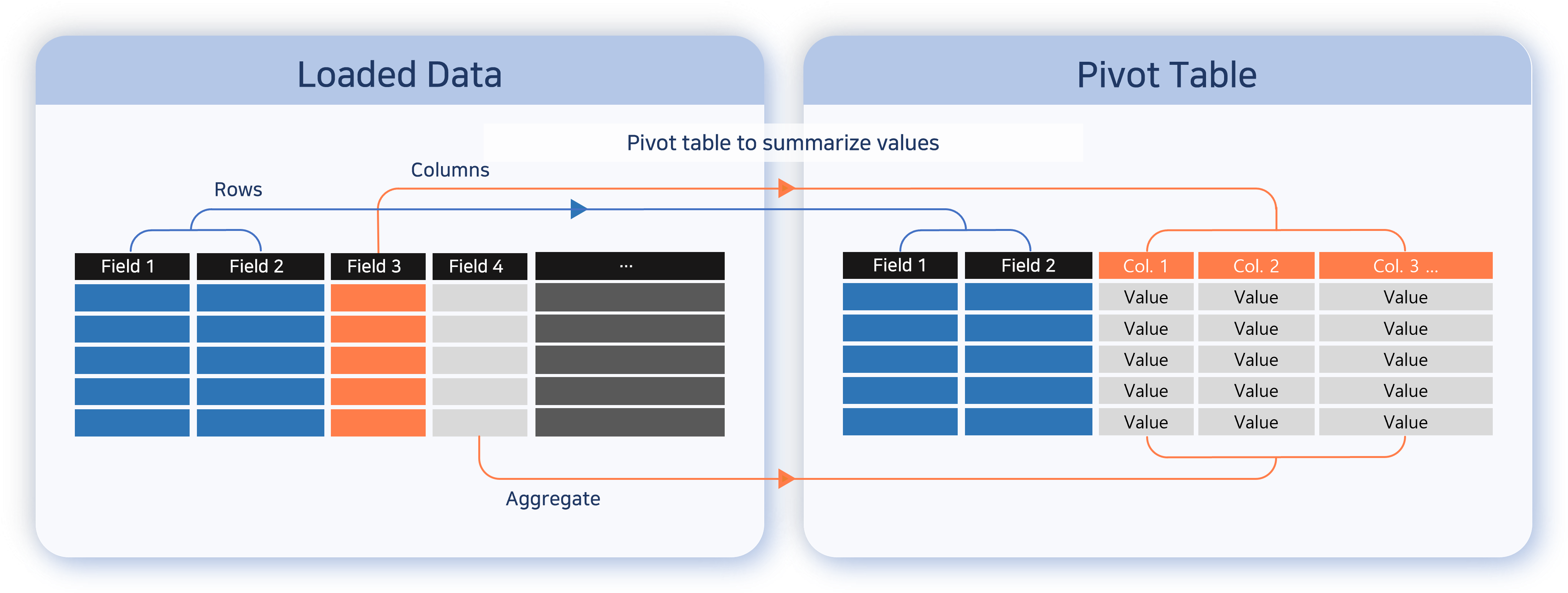
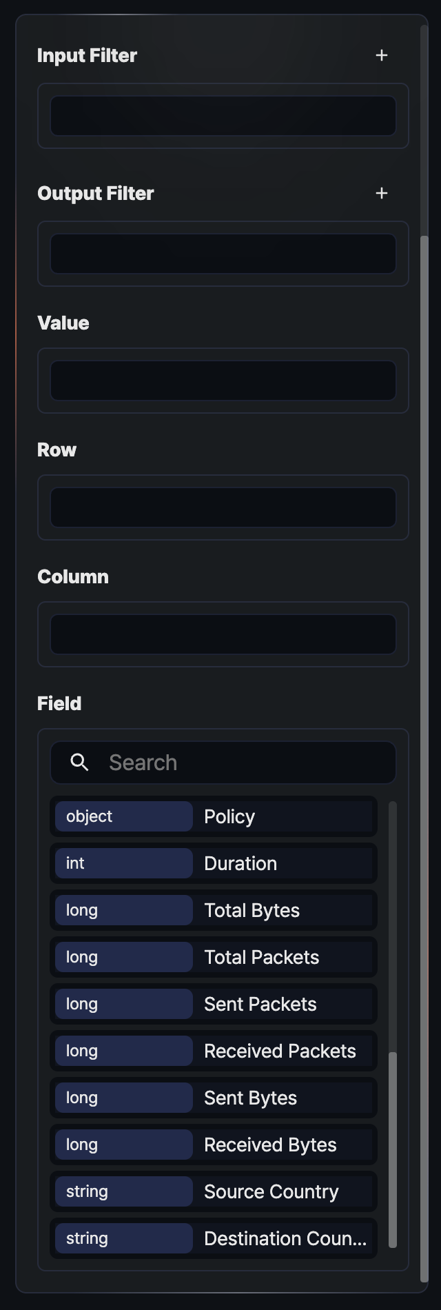
Field list and placement areas
The left analysis-tool panel is organized top to bottom as Input Filter, Result Filter, Values, Rows, Columns, and Fields.
- Input Filter: A preprocessing filter applied before aggregation. Records filtered out here are excluded from every later stage.
- Result Filter: A post-processing filter applied only to the results after values, rows, and columns have been aggregated. A
limitfilter that caps results at 10,000 is included by default. - Values: The fields to be aggregated. They are used with aggregation functions (count, sum, and so on). Pivot mode is activated once at least one field is placed in the Values area.
- Rows: The fields used to group the aggregated result as rows. Placing multiple fields creates a hierarchical grouping.
- Columns: The fields used to group the aggregated result as columns. Combined with rows, they build a cross-aggregation table.
- Fields: The list of original fields from the loaded data. Each field shows its data type on the left; drag an item to Values, Rows, or Columns to place it. The Count item at the top of the list is a default aggregation that counts total rows without a field, and can be placed only in the Values area.
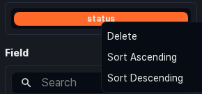
Clicking a field item directly opens a dropdown menu with filter and sort options for that field. Filters added through this path are always registered as input filters.
Input filters
Use an input filter when you want to reduce the original records before aggregation. Applying the condition before loading everything into memory speeds up processing and prevents distortion caused by unneeded data.
Click the ![]() button on the right of the Input Filter header to choose between Standard Filter and Dynamic Filter. Dynamic Filter is visible only to accounts with permission to view user-defined variables.
button on the right of the Input Filter header to choose between Standard Filter and Dynamic Filter. Dynamic Filter is visible only to accounts with permission to view user-defined variables.
Standard filter
Use this option when you want to apply an advanced condition by writing a Logpresso query directly. You can express boolean value comparisons that are hard to write with plain comparison operators, function calls such as contains(), and combinations of multiple conditions.
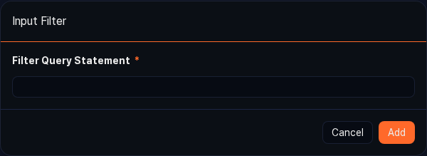
- Click the
 button in the Input Filter header, and then select Standard Filter.
 - In the Query field, enter the query to use as the filter (for example,
search status == 200). - Click Add to register the filter in the input filter list.
Dynamic filter
Use a dynamic filter when you want to use a value received from a dashboard input-control widget as the filter condition. Specify the target field, user-defined variable, and comparison condition through the form, and the query is generated and registered as a filter automatically.
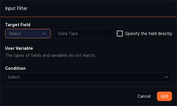
- Target field: The field the filter applies to. Choose from the field list, or select the Enter field manually check box to enter the field name and type directly.
- User-defined variable: A variable passed in from the dashboard input-control widget. Click the
 button to refresh the list, or click the
  Settings button to open the User-Defined Variables page in a new window and add a variable.
 - Condition: The operator used to compare the target field value (left operand) with the user-defined variable value (right operand). The available operators depend on the data type of the target field.
Result filters
Use a result filter when you want to apply a condition on top of the aggregated result. For example, a condition like "show only rows with count of 100 or more" works on aggregated values and cannot be expressed with an input filter; it can only be expressed with a result filter.
Click the ![]() button on the right of the Result Filter header to add a Standard Filter or Dynamic Filter. The method and input fields are the same as for input filters.
button on the right of the Result Filter header to add a Standard Filter or Dynamic Filter. The method and input fields are the same as for input filters.
Standard filter
Write a query directly, the same way as for the input filter's standard filter. A query registered as a result filter is applied to the result records after aggregation.
Dynamic filter
Use the same form as the input filter's dynamic filter; the only difference is that the filter is registered in the result filter area.
Limiting result count
The result filter area includes a limit filter by default that caps the result at 10,000 records. This filter is a safeguard to keep the browser responsive by preventing a large result set from being sent to it.
Click the ![]() icon on the right of a filter to remove it. This applies to both input and result filters.
icon on the right of a filter to remove it. This applies to both input and result filters.
Placing values
The Values area is what the pivot aggregates. When you drag a field from the field list to the Values area, a default aggregation function is applied automatically: sum for numeric fields and count for the rest. If you drag the default Count item, count() is registered with no specific field, counting every row.
Changing the aggregation function
Click a placed value item to open a popover for choosing the aggregation function. Select a function from the list on the left to see its description on the right, then click Edit to replace the current function with the selected one.
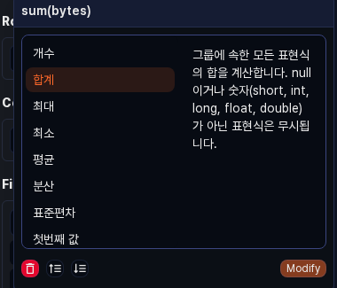
The following aggregation functions are available:
| Function | Description |
|---|---|
count | Counts the rows in each group. If an expression is provided, returns only the count of rows whose value is not null. |
sum | Calculates the sum of every expression in a group. Non-numeric values and null are ignored. |
max | Returns the maximum expression value in a group. null is ignored. |
min | Returns the minimum expression value in a group. null is ignored. |
avg | Calculates the average of every expression in a group. Non-numeric values and null are ignored. |
var | Calculates the variance of every expression in a group. Non-numeric values and null are ignored. |
stddev | Calculates the standard deviation of every expression in a group. Non-numeric values and null are ignored. |
first | Returns the first expression value in a group. |
last | Returns the last expression value in a group. |
values | Returns the set of distinct values in a group as an array. Collects up to 100 values per group. |
dc | Returns the number of distinct values. |
estdc | Returns an estimate of the number of distinct values. Use this to get an approximate value faster than dc on large data sets. |
At the bottom of the popover you can click the ![]() button to remove the value item, or click the ascending or descending sort buttons to sort the result by the current aggregation value.
button to remove the value item, or click the ascending or descending sort buttons to sort the result by the current aggregation value.
Renaming a value field
Double-click a placed value item to turn it into an editable input box. Enter a new name and press Enter to apply the change, or press Esc to cancel editing. The new name is reflected in the result grid and in the generated query's as clause.
Removing and sorting a value field
Click a value item to open the popover, where you can perform the following actions:
- Delete: Click the
 button to remove the aggregation item from the Values area.
 - Ascending/Descending sort: Click the sort button to add a
sortfilter for the current aggregation value. Ascending sorts from small values to large; descending, from large to small.
Placing rows
Drag a field from the field list to the Rows area to group records by the field's values. Placing multiple fields creates a hierarchical grouping where the first field is the parent group and the next field is its child group.
Sorting, removing, and renaming a row
Clicking a placed row item opens a dropdown with the following menu items:
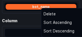
- Delete: Removes the field from the Rows area.
- Ascending: Adds an ascending sort filter based on the field's value.
- Descending: Adds a descending sort filter based on the field's value.
As in the Values area, you can rename an item by double-clicking it to switch to the edit box and entering a new name.
Rearranging rows
Drag an item within the Rows area to change its order. Because the field at the top becomes the parent group, adjust the order and run again when changing the analysis angle. If you drag an item from the Rows area to the Columns or Values area, it moves to that area and is removed from Rows.
Placing columns
Drag a field from the field list to the Columns area to expand the field's values as column headers and build a cross-aggregation table. For example, placing the src_ip field in Rows, status in Columns, and Count in Values lets you see the distribution of HTTP status codes per IP at a glance.
Sorting, removing, and renaming a column
Clicking a placed column item opens the same dropdown menu as in the Rows area, with Delete, Ascending, and Descending.
Double-click an item to rename its display name.
Rearranging columns
Drag an item within the Columns area to change its order. If you drag an item from the Columns area to the Rows or Values area, it moves to that area. Use this to quickly swap rows and columns.
Searching fields
When the field list is long and you have trouble finding a field, use the search box at the top of the list. Only fields that match the entered string are highlighted. The search is case-insensitive and uses partial matching on the field name. You can drag a field from the search result directly to the Values, Rows, or Columns area.
Analyzing data
Once the pivot table is configured, you can explore the aggregated result in the grid, inspect a cell for details, or switch to the chart view for a visual sense of the distribution. Combining data from multiple tabs with a join or union correlation analysis helps you find threat signs in relationships between different logs. A common usage pattern is to summarize a large volume of events quickly to spot anomalies, then drill down to the Logs or Events page to check the evidence.
Viewing the pivot table
When a query runs, the result appears in a grid by default. The grid view is active when the ![]() button on the left of the toolbar is highlighted. From the grid, you can right-click a column header or cell to run various analysis actions.
button on the left of the toolbar is highlighted. From the grid, you can right-click a column header or cell to run various analysis actions.
Column header menu
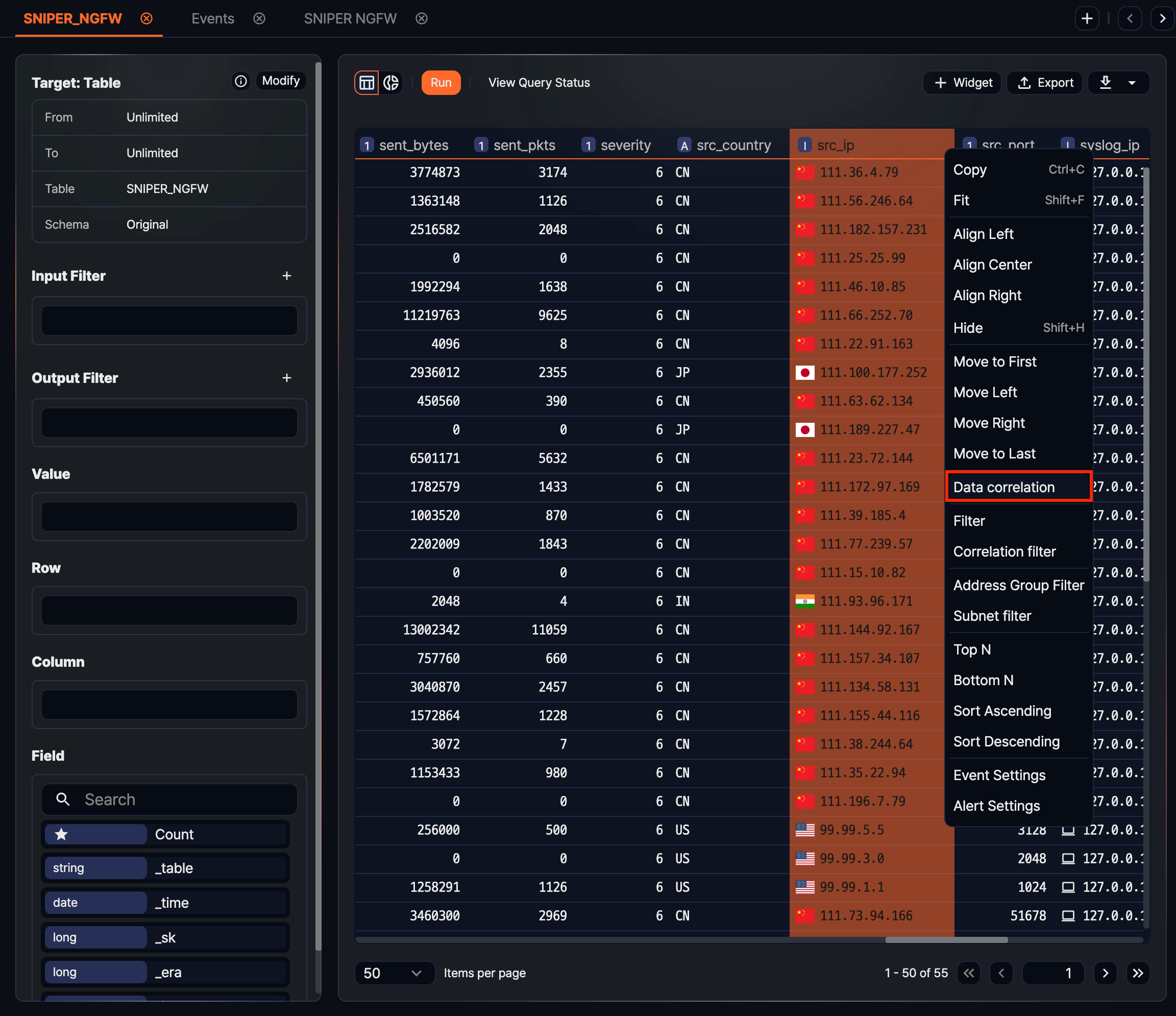
Click a column header to rearrange data by that column or to build derived queries such as filters, sorts, and top-N extractions. Some items are hidden depending on the column type (string, number, date, and so on).
- Copy: Copies the selected column's values as tab-separated text to the clipboard (shortcut: Ctrl + C).
- Fit: Automatically adjusts the column width to fit the cell content (shortcut: Shift + F).
- Align left, Align center, Align right: Changes the cell content's alignment.
- Hide: Hides the selected column from the result grid (shortcut: Shift + H).
- Move to start, Move left, Move right, Move to end: Changes the display order of the column. If the current column is already at the far left, the left-related items are hidden; if it is at the far right, the right-related items are hidden.
- Correlation analysis: Runs a correlation analysis against data in another tab using the column's values. For details, see Correlation analysis.
- Filter condition: Sets a condition on the selected column to filter the result. You can specify comparison operators, values, and combinations of multiple conditions (AND/OR) in a dialog.
- Correlation filter: Filters the current result by the result in another tab. Use it to keep only the values present in both data sets or to isolate values that exist in only one side.
- Truncate by time unit: Truncates a date-type column's values to the specified unit (second, minute, hour, day, month, and so on) into a new field. Use it to build aggregations by time bucket.
- Calculate time difference: Creates a new field that computes the difference between two date fields. Use it to build metrics such as event intervals or dwell time.
- String transformation: Applies transformations to a string-type column, such as case conversion, whitespace removal, or substring extraction, into a new field.
- Top N, Bottom N: Keeps only the top or bottom N records by the column's values. Clicking opens a dialog for specifying N.
- Ascending, Descending: Sorts the result by the column. Reflected in the query as the sort command.
- Thousands separator: Applies the thousands separator to a numeric column. A check icon is shown when enabled. Useful for reading large numbers at a glance.
- Event setting: Configures value changes of the column to be the trigger for an event. For details, see Event setting.
- Alert setting: Configures an alert to fire when the column's value meets a threshold. For details, see Alert setting.
Cell context menu
Right-clicking a cell lets you trace the source of the value, diagnose it against external threat intelligence, or use the cell value itself as a filter condition for deeper analysis. The items shown depend on the cell type, as follows.
All data cells (not the header)
- Decode: Shows the decoded result of the selected cell or of a substring dragged inside the cell. Use it to unwrap Base64- or URL-encoded parameters or payloads in place.
IP type cells
Shown only on cells that are fields normalized to an IP address. IPs stored as strings in the logger or table source must be normalized to the IP type through a schema for this item to appear.
-
Search last 10 minutes: Queries other events that contain the same IP within 10 minutes before or after the event time (related command: fulltext). If the result has no time field, the search uses the last 10 minutes from the current time.
-
Add to IP blocklist: Registers the selected IP value in an address group. Useful for managing recurring malicious IPs as a blocklist or for reusing them as conditions in detection rules.
-
Look up in VirusTotal: Opens the VirusTotal diagnostic page for the selected IP in a new window. Use it to quickly check the reputation of a suspicious address.
NoteLook up in VirusTotal is not available in an isolated network where outbound connections are blocked.
Cells with an original event identifier
Shown only when the record contains an original event identifier (event GUID), such as when querying events generated by a detection rule.
- View original event: Opens the detail window of the original event linked to the aggregated record. Use it to see which original records contributed to a summarized result.
Cells that support value comparison
Shown on cells of string, number, or date types where comparison operators are defined. The operators actually shown depend on the cell type.
- Cell value filter: Adds a filter comparing against the current cell value (equal, not equal, contains, greater than or equal, less than or equal, and so on). For example, you can click once to apply "keep only rows with this attacker IP" or "exclude this value."
Grid display options
Click the row number area header (the leftmost column) to adjust the overall display of the grid. Selected options are marked with a check icon.
- Show stripes: Applies alternating background colors to odd and even rows to emphasize row boundaries.
- Show borders: Shows dividers between cells.
- Reduce cell spacing: Narrows row spacing so more rows fit on the screen.
- Adjust column width: Allows column widths to be adjusted by dragging.
Page navigation
Use the page navigation controls at the bottom of the grid to browse other pages of the result set. The total page count and the current page number are shown, and you can type a page number directly into the input field to jump there. The number of records shown per page follows the page size at the time the query was run.
Viewing charts
Visualizing the aggregated result directly as a bar, line, or pie chart lets you see large swings or skewed distributions without reading every number. Because the chart view shares the same query result as the grid view, changes to the pivot configuration (rows, columns, values) update the chart immediately.
Switching to the chart
Click the ![]() button on the left of the toolbar to switch from the grid view to the chart view. Click the
button on the left of the toolbar to switch from the grid view to the chart view. Click the ![]() button to return to the grid. You can switch to the chart view only when at least one field is placed in the Rows area.
button to return to the grid. You can switch to the chart view only when at least one field is placed in the Rows area.

Chart settings
In the chart view, click the ![]() button to open the Widget Settings dialog, where you can pick the chart type and visualization options.
button to open the Widget Settings dialog, where you can pick the chart type and visualization options.

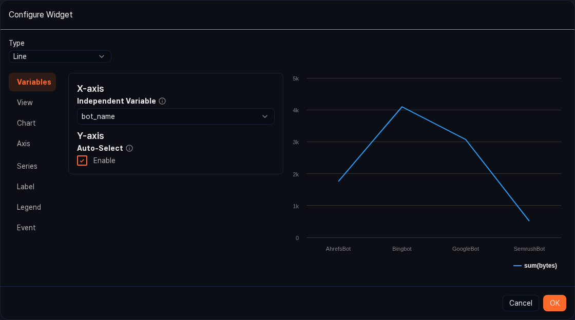
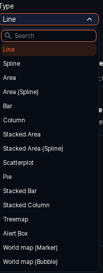
-
Type: Choose the chart type that best fits the distribution of the data. Available types are Line, Spline, Area, Area (Spline), Bar, Column, Stacked Area, Stacked Area (Spline), Scatterplot, Pie, Stacked Bar, Stacked Column, Treemap, Alert Box, World Map (Marker), and World Map (Bubble).
-
Event setting: Configures the display condition of events on the chart. When the alert box type is selected, specify the block condition, message text, sound notification, and so on.
-
Visualization options: Depending on the selected chart type, detailed options such as X-axis and Y-axis fields, legend position, and colors are shown dynamically. Click OK when finished to apply the result.
Correlation analysis
Loading data from different security devices into a single pivot session and joining it by a common field can expose relationships that are invisible in each log alone. For example, combining firewall block logs with web server access logs on the same source IP shows which URLs an IP with a block history has been targeting, all on one screen.
Six correlation types are available depending on how the data sets are combined. Choose the type that matches your goal so that only the records you want remain in the result.
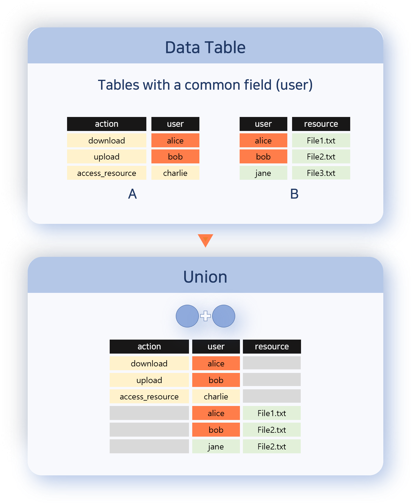
Union
Merges all records from both data sets into a single output. Matching on the correlation field is not checked, and each record is kept as-is. Use this when you want to look at the two data sets combined into one. Record order is not guaranteed.
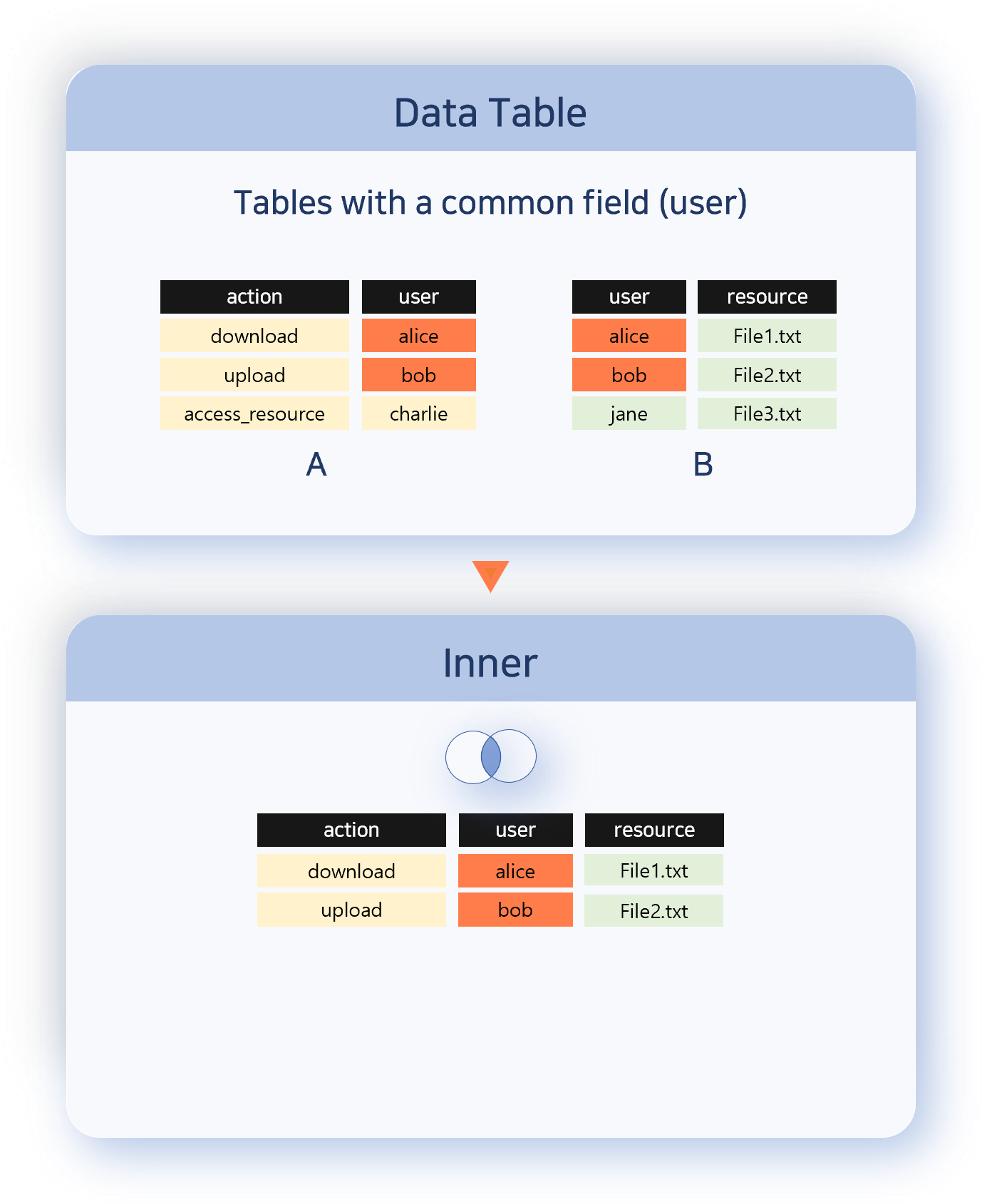
Inner
Outputs only the records with matching correlation field values from both data sets. Use this when you want to analyze only the common items (the intersection) of the two sets.
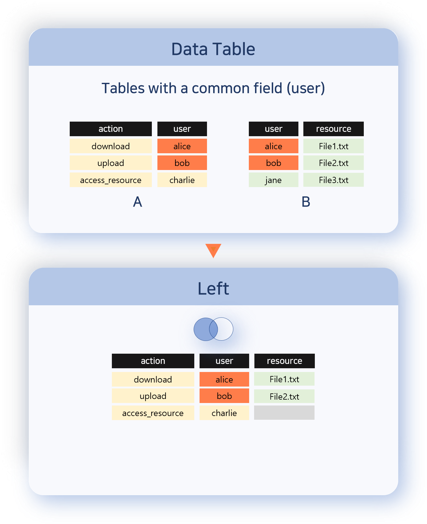
Left
Keeps every record from the left data set and attaches information from the right when a correlation field value matches. Use this when you want to preserve the reference set (left) while adding auxiliary information.
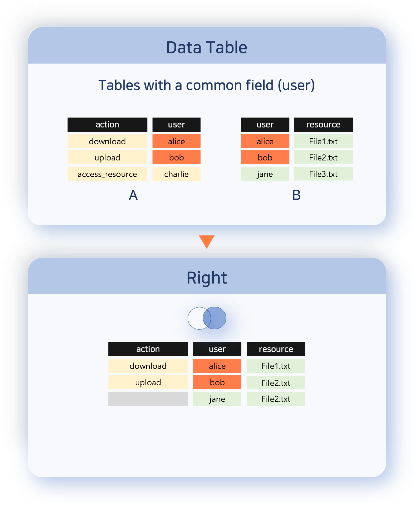
Right
Keeps every record from the right data set and attaches information from the left when a correlation field value matches. The direction is opposite of Left.
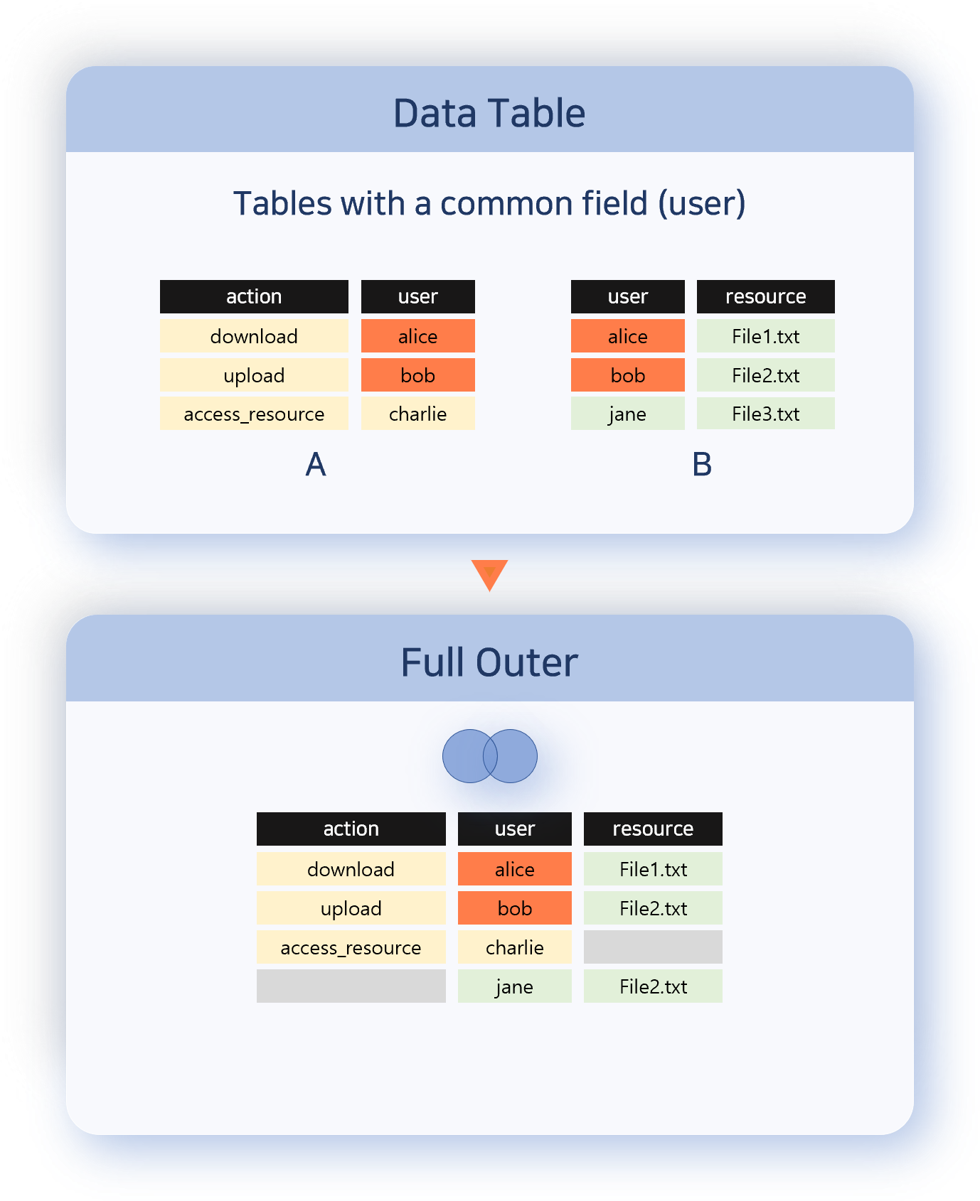
Full Outer
Outputs every record from both data sets. Records with matching correlation field values are combined into a single row; those without a match are kept as-is from each set. Use this when you need to see missing items from both sides.
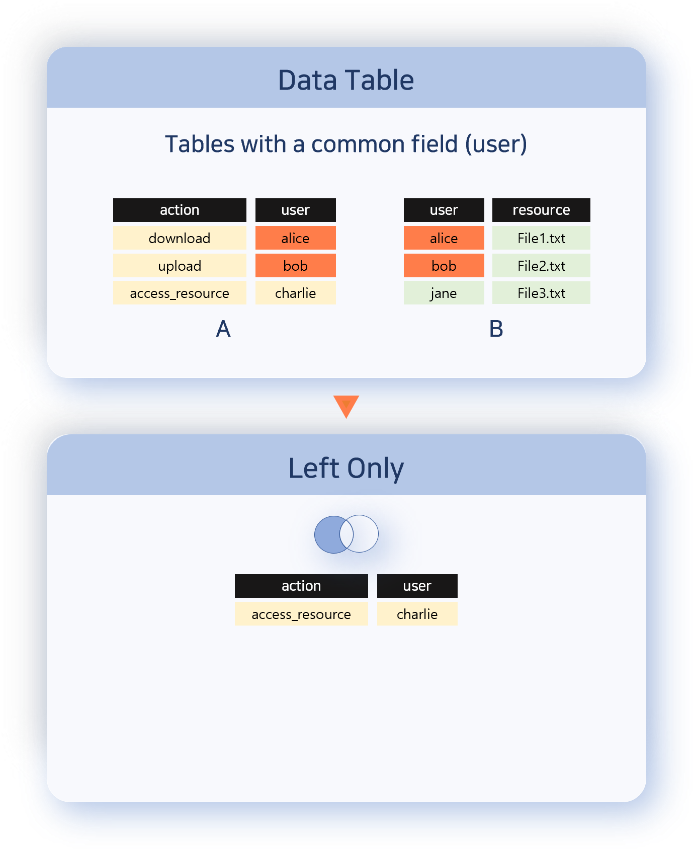
Left Only
Outputs only the records from the left data set whose correlation field value does not match any in the right set. The opposite of Inner; useful for finding items that appear only on one side or that are missing.
Analysis procedure
The following example combines an address group that contains attacker IPs with web server logs to aggregate the attack status against the web server.
-
Prepare the data to analyze. Open two or more pivot tabs, load the data in each, and rename the tabs to reflect their content.
-
Right-click the header of the column that will be the correlation key (for example, src_ip in the web server logs), and click Correlation analysis in the pop-up menu.
-
In the Add correlation analysis dialog, set the following items and click OK.
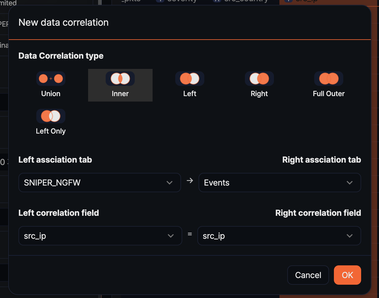
- Correlation analysis type: Choose Union, Inner, Left, Right, Full Outer, or Left Only.
- Left tab: Select the pivot tab to use as the left data set.
- Right tab: Select the pivot tab to use as the right data set.
- Left correlation field: Select the field from the left tab to compare the two sets. Not shown when the type is Union.
- Right correlation field: Select the field from the right tab to compare the two sets. Not shown when the type is Union.
-
Configure the Rows, Columns, and Values areas over the combined result as in a regular pivot table to aggregate it into the form you want.
Viewing query status
Click View query status on the right of the toolbar to expand the execution-status panel of the current query below the grid. The button is highlighted when the panel is open; click it again to collapse it. When a query is slower than expected or the result count differs from what you expected, use this panel to see which stage is taking time and how many records were processed, so you can adjust the query configuration. For details on each field, see Query Monitor.
Reusing analysis results
Analysis results in Pivots are not limited to one-off queries; they can be reused in various ways. SOC analysts can reduce repeated work and connect analysis results to dashboards, tickets, and external tools to carry the detection-analysis-response flow forward.
Use any of the following approaches:
- Save as dataset: Reuse the result as the common base data for multiple widgets or repeated analyses.
- Save query result: Preserve a snapshot of the result on the server so it can be queried later.
- Download as a file: Download as CSV, JSON, and so on for external reports or offline analysis.
- Add as a widget: Place it on a dashboard to build a real-time monitoring screen.
- Export as a pivot file: Share the same analysis setup with another Sonar system or with fellow analysts.
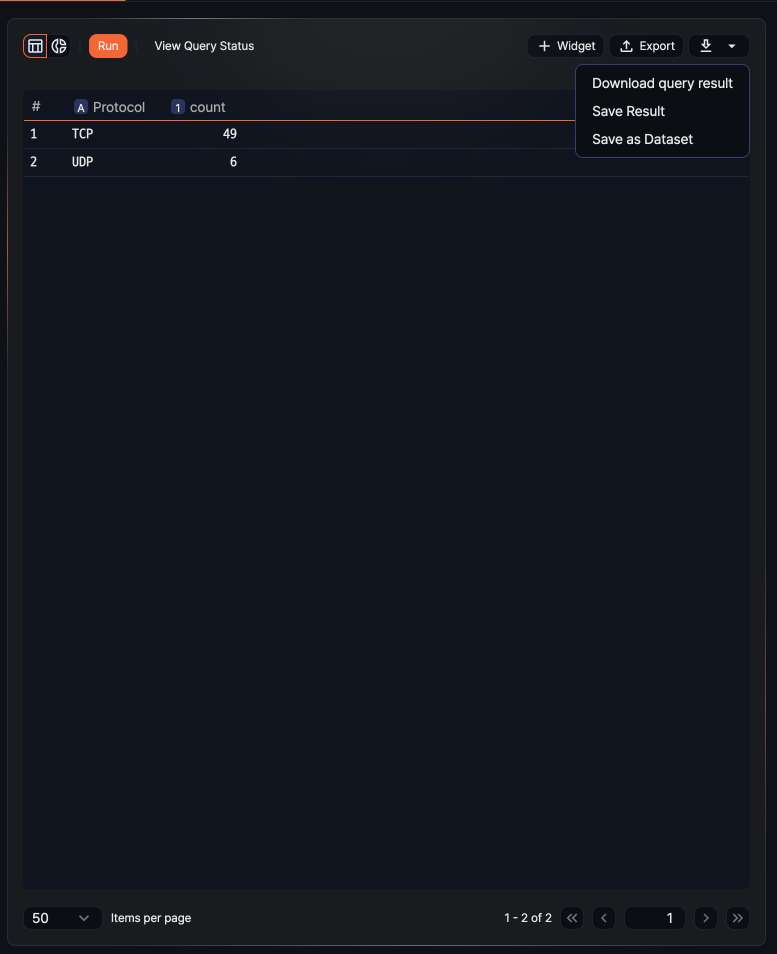
Hovering over the ![]() icon in the toolbar opens a menu with Download Result, Save Result, and Save as Dataset. Add widget and export pivot have their own separate buttons.
icon in the toolbar opens a menu with Download Result, Save Result, and Save as Dataset. Add widget and export pivot have their own separate buttons.
Save as dataset
Saving an analysis result as a dataset lets you share the same query across multiple widgets or reuse it as the base for other pivot analyses. It is convenient for analysis conditions you need to query repeatedly.
-
Shape the data into a form suitable for saving as a dataset. Use a Recent range (for example, the last 1 hour), and remove the result filter that limits the record count if needed.
-
In the toolbar, open the dropdown of the
 icon and click Save as Dataset.
 -
In the Add dataset dialog, fill in the fields and click Add.
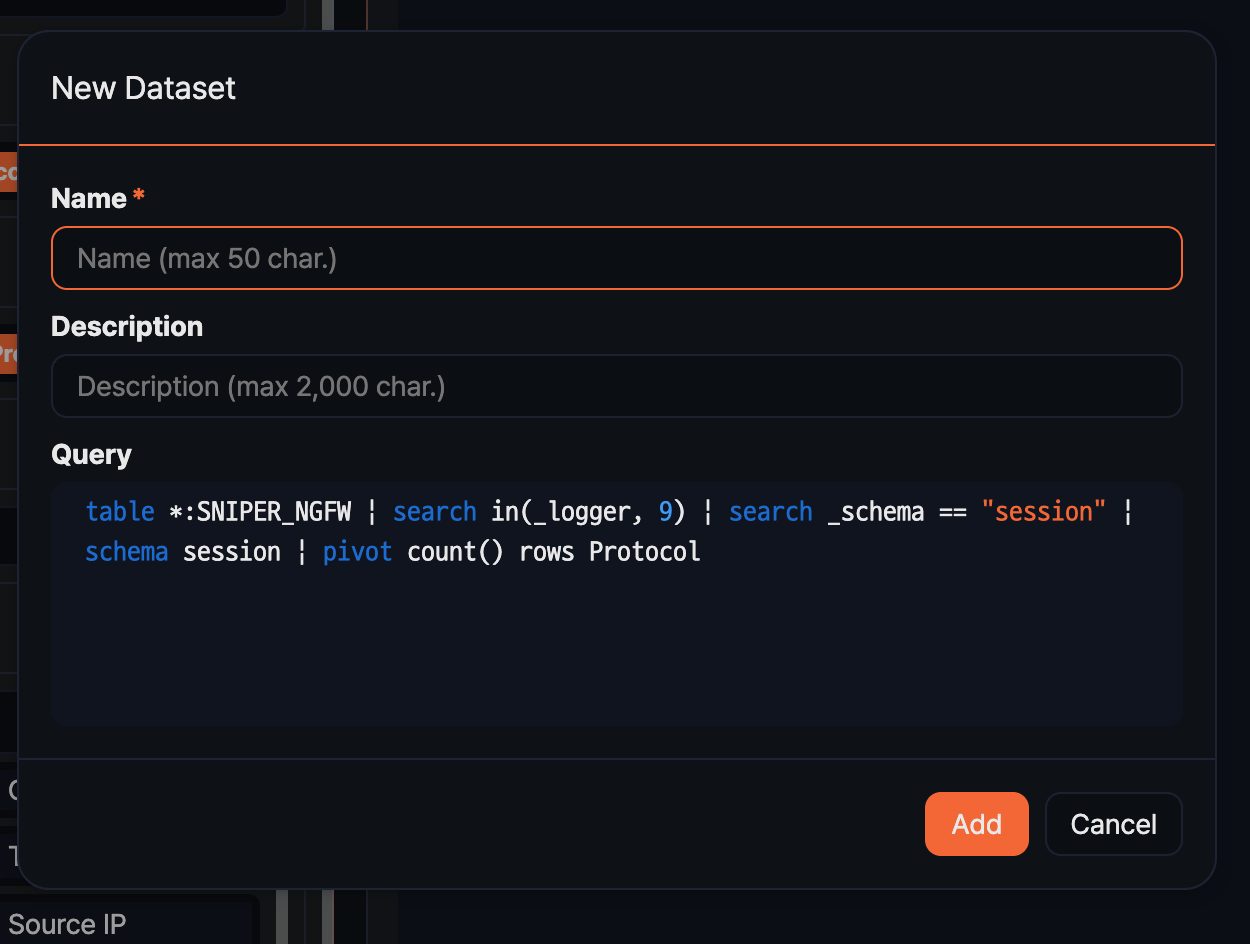
- Name: Dataset name (required, up to 50 characters)
- Description: A description of the dataset's purpose or criteria (up to 2,000 characters)
- Query: Filled in automatically with the query generated from the current pivot configuration. It cannot be edited here.
You can review and edit the saved dataset from the Analysis > Datasets menu.
Save query result
To preserve an analysis result at a specific point in time as a snapshot, save the query result. Because the saved result lives on the server, you can view it later exactly as it was at the time of the analysis, even if the underlying data changes. Useful as evidence for incident investigations or report writing.
-
In the toolbar, open the dropdown of the
icon and click Save Result. -
In the Save Query Result dialog, enter a Name (required, up to 100 characters) and click OK.
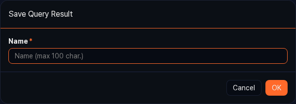
You can view the saved result from Analysis > Queries > Load query result.
Download query result
You can download the analysis result to your local PC as a file and use it in external analysis tools or in reports.
-
In the toolbar, open the dropdown of the
icon and click Download Result. -
In the Download Query Result dialog, set the fields and click Download.
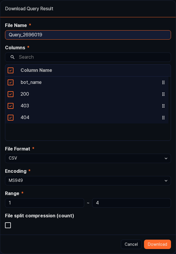
- File name: Name of the file to save (required, default:
Query_{query_number}) - Columns: Select the fields to include in the file. All fields are selected by default.
- File format: The export format (default: CSV, range: CSV, XML, Microsoft Word, HTML, JSON, PDF)
- File encoding: Text encoding (shown only when the file format is CSV or JSON; the default depends on the current language, range: UTF-8, UTF-16, MS949, and so on)
- Range: Specify the row range to download as
start~end. - Save as split ZIP: Shown only when the file format is CSV. Select it to split the file into the specified number of records and bundle them in a ZIP.
- File name: Name of the file to save (required, default:
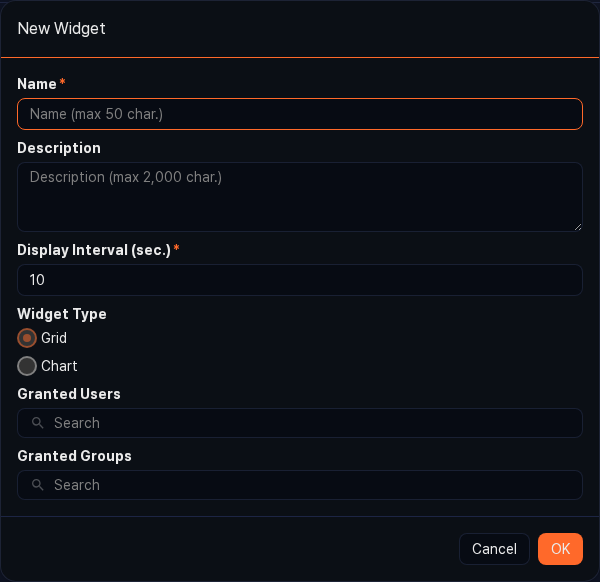
Add widget
The pivot analysis page composes data the same way as the widget editing page, so you can turn the analysis result directly into a widget and place it on a dashboard. Register metrics you need to monitor in real time as widgets, and you can see the latest values without running the query separately.
-
Use Grid view or Chart view to shape the data into the form you want.
-
Click Add Widget in the toolbar.
-
In the Add Widget dialog, fill in the fields and click OK.
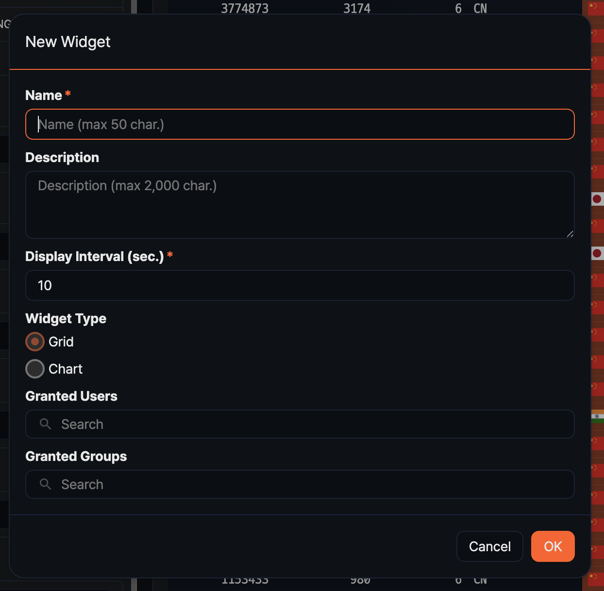
- Name: Widget name (required, up to 50 characters)
- Description: A description of the widget's purpose (up to 2,000 characters)
- Interval: Interval for automatic refresh, in seconds (default:
10, range: 1 to 2,147,483). Set a generous value for queries with large data volume to reduce load. - Widget type: Choose Grid or Chart (default depends on the current view).
- Shared accounts / Shared groups: Select the accounts or account groups to share the widget with. If none is selected, only you can view it.
You can view and edit the added widget from Dashboard > Widget Management.
Grid widget
Adding a widget from the Grid view creates a grid widget that displays the analysis result as a table. Useful for quickly scanning a large number of rows or for highlighting cell colors based on field values. Grid widgets support per-column event and alert settings.
Right-clicking a column header in the grid shows the Event setting and Alert setting menu items.
Chart widget
Adding a widget from the Chart view creates a chart widget that visualizes the data. Useful for understanding trends over time or ratios across items at a glance.
Change chart type, colors, axis configuration, and so on through the Settings button in the chart toolbar. For recommended uses of each chart type, see the Analyzing data > Chart settings section.
Event setting (per column)
In a grid widget, configure the action to run when a user clicks a cell. For example, clicking an IP address cell can apply the IP as a filter or run a related query in a new window. Setting events shortens investigation time by leading directly from the dashboard to detailed analysis.
-
In the grid, right-click the header of the target column and click Event setting.
-
In the Event setting dialog, choose the action to run and click Apply.
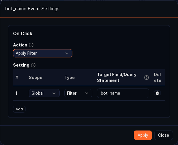
- Apply filter: Applies the cell value as a global dashboard filter.
- Run query: Runs the specified query in a new query window. The cell value can be referenced in the query using the
$field_name$macro. - Open browser: Opens a new browser window with the cell value as the URL. Useful when the field contains a URL.
- Navigate page: Navigates to the specified URL within the current web console.
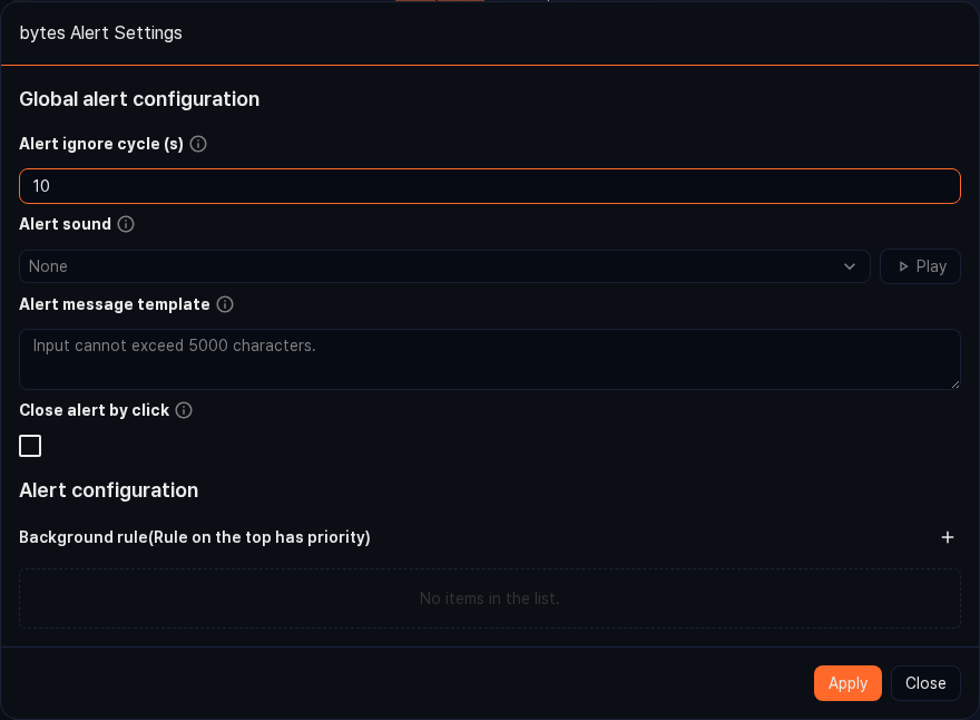
Alert setting (per column)
In a grid widget, you can highlight a cell's color and trigger a sound or browser notification when a specific column value crosses a configured threshold. Useful for real-time monitoring screens where you need to quickly notice values outside the normal range.
-
In the grid, right-click the header of the target column and click Alert setting.
-
In Common settings of the Alert setting dialog, configure the notification behavior. Sound, notification message template, alert-ignore interval, and so on are set here.
-
In the Conditions area, add conditions one by one, each with a comparison operator, threshold, text and background color, and whether to notify, then click Apply.
Export pivot
Exporting the current pivot configuration as a .pivot file lets you transfer the same analysis setup to another Sonar system as is, or share it with fellow analysts. Only the analysis setup (data source, fields, filters, pivot configuration, and so on) is saved, not the data itself, so the file size is small.
-
In the toolbar, click Export.
-
In the Export pivot dialog, enter a Name (required) and click Export. The
.pivotextension is added automatically.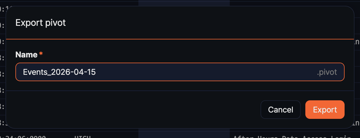
Import pivot
Importing a .pivot file restores a pivot with the same analysis setup. Because the data query time uses the import time as its reference point, a range saved as Last 1 day queries the last 1 day of data from the import time.
-
On the Analysis > Pivots page, click the Import button in the toolbar (or the Import Pivot button in the center of the empty screen).
-
In the Import Pivot dialog, select the
.pivotfile and click OK.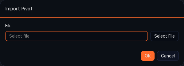
If some of the data sources referenced by the imported file do not exist on the current system, or include items the account does not have access to, an Import Pivot Result report is shown. The report lists the missing items' Type, Name, and Reason in a table, so you can see at a glance which sources need to be recovered.
Import may fail in the following situations:
- The logger, table, dataset, or behavior profile used at export time no longer exists on the current system.
- A table with the same name as at export time does not exist.
- The current account does not have access to a data source included in the pivot file.
- The file is corrupted or its extension is not
.pivot.
If only some sources are missing, the import continues using the items that do exist.
Toolbar
After data is loaded, the toolbar at the top of the screen lets you rerun the current pivot result or continue with other actions.

- Run: Reruns the current pivot configuration. You need to click this button to apply changes to value, row, or column placement or to filters.
- View query status: Shows the status of the running task and the query that Logpresso generated.
- Widget: Starts the flow for saving the current result as a widget. Use it to build metrics you want to check periodically on a dashboard.
- Export: Saves the current pivot configuration as a
.pivotfile.